This document is relevant for: Trn2, Trn3
Tensor Indexing on NKI#
This topic covers basic tensor indexing and how it applies to developing with the AWS Neuron SDK. This overview describes basic indexing of tensors with several examples of how to use indexing in NKI kernels.
Basic Tensor Indexing#
NKI supports basic indexing of tensors using integers as indexes. For example, we can index a 3-dimensional tensor with a single integer to get a view of a portion of the original tensor.
x = nl.ndarray((2, 2, 2), dtype=nl.float32, buffer=nl.hbm)

# `x[1]` return a view of x with shape of [2, 2]
# [[x[1, 0, 0], x[1, 0 ,1]], [x[1, 1, 0], x[1, 1 ,1]]]
assert x[1].shape == [2, 2]
NKI also supports creating views from sub-ranges of the original tensor dimension. This is done with the standard Python slicing syntax. For example:
x = nl.ndarray((2, 128, 1024), dtype=nl.float32, buffer=nl.hbm)

# `x[1, :, :]` is the same as `x[1]`
assert x[1, :, :].shape == [128, 1024]

# Get a smaller view of the third dimension
assert x[1, :, 0:512].shape == [128, 512]

# `x[:, 1, 0:2]` returns a view of x with shape of [2, 2]
# [[x[0, 1, 0], x[0, 1 ,1]], [x[1, 1, 0], x[1, 1 ,1]]]
assert x[:, 1, 0:2].shape == [2, 2]
When indexing into tensors, NeuronCore offers much more flexible memory access in its on-chip SRAMs along the free dimension. You can use this to efficiently stride the SBUF/PSUM memories at high performance for all NKI APIs that access on-chip memories. Note, however, this flexibility is not supported along the partition dimension. That being said, device memory (HBM) is always more performant when accessed sequentially.
Tensor Indexing by Example#
In this section, we share several use cases that benefit from advanced memory access patterns and demonstrate how to implement them in NKI.
Case #1 - Tensor split to even and odd columns#
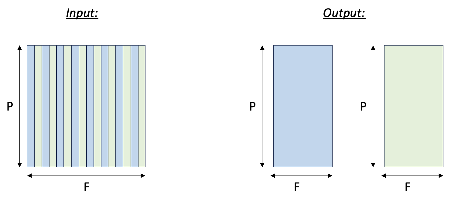
Here we split an input tensor into two output tensors, where the first output tensor gathers all the even columns from the input tensor, and the second output tensor gathers all the odd columns from the input tensor. We assume the rows of the input tensors are mapped to SBUF partitions. Therefore, we are effectively gathering elements along the free dimension of the input tensor. The figure below visualizes the input and output tensors.
Tensor split to even and odd columns
 1import nki
 2import nki.language as nl
 3import math
 4
 5@nki.jit
 6def tensor_split_kernel_(in_tensor):
 7  """NKI kernel to split an input tensor into two output tensors, along the column axis.
 8
 9  The even columns of the input tensor will be gathered into the first output tensor,
10  and the odd columns of the input tensor will be gathered into the second output tensor.
11
12  Args:
13      in_tensor: an input tensor
14  Returns:
15      out_tensor_even: a first output tensor (will hold the even columns of the input tensor)
16      out_tensor_odd: a second output tensor (will hold the odd columns of the input tensor)
17  """
18
19  # This example only works for tensors with a partition dimension that fits in the SBUF
20  assert in_tensor.shape[0] <= nl.tile_size.pmax
21
22  # Extract tile sizes.
23  sz_p, sz_f = in_tensor.shape
24  sz_fout_even = sz_f - sz_f // 2
25  sz_fout_odd = sz_f // 2
26
27  # create output tensors
28  out_tensor_even = nl.ndarray((sz_p, sz_fout_even), dtype=in_tensor.dtype, buffer=nl.shared_hbm)
29  out_tensor_odd = nl.ndarray((sz_p, sz_fout_odd), dtype=in_tensor.dtype, buffer=nl.shared_hbm)
30
31  # Load input data from external memory to on-chip memory
32  in_tile = nl.load(in_tensor)
33
34  # Store the results back to external memory
35  nl.store(out_tensor_even, value=in_tile[:, 0:sz_f:2])
36  nl.store(out_tensor_odd,  value=in_tile[:, 1:sz_f:2])
37
38  return out_tensor_even, out_tensor_odd
39
40
41if __name__ == "__main__":
42    import torch
43    import torch_xla
44
45    device = torch_xla.device()
46
47    X, Y = 4, 5
48    in_tensor = torch.arange(X * Y, dtype=torch.bfloat16).reshape(X, Y).to(device=device)
49
50    out1_tensor, out2_tensor = tensor_split_kernel_(in_tensor)
51    print(in_tensor, out1_tensor, out2_tensor)
The main concept in this example is that we are using slices to access the even and odd columns of the input tensor. For the partition dimension, we use the slice expression :, which selects all of the rows of the input tensor. For the free dimension, we use 0:sz_f:2 for the even columns. This slice says: start at index 0, take columns unto index sz_f, and increment by 2 at each step. The odd columns are similar, except we start at index 1.
Case #2 - Transpose tensor along the f axis#
In this example we transpose a tensor along two of its axes. Note, there are two main types of transposition in NKI:
Transpose between the partition-dimension axis and one of the free-dimension axes, which is achieved via the nki.isa.nc_transpose API.
Transpose between two free-dimension axes, which is achieved via a nki.isa.dma_copy API, with indexing manipulation in the transposed axes to re-arrange the data.
In this example, we’ll focus on the second case: consider a
three-dimensional input tensor [P, F1, F2], where the P axis is mapped
to the different SBUF partitions and the F1 and F2 axes are
flattened and placed in each partition, with F1 being the major
dimension. Our goal in this example is to transpose the F1 and
F2 axes with a parallel dimension P,
which would re-arrange the data within each partition. The figure below illustrates the input and output tensor layouts.
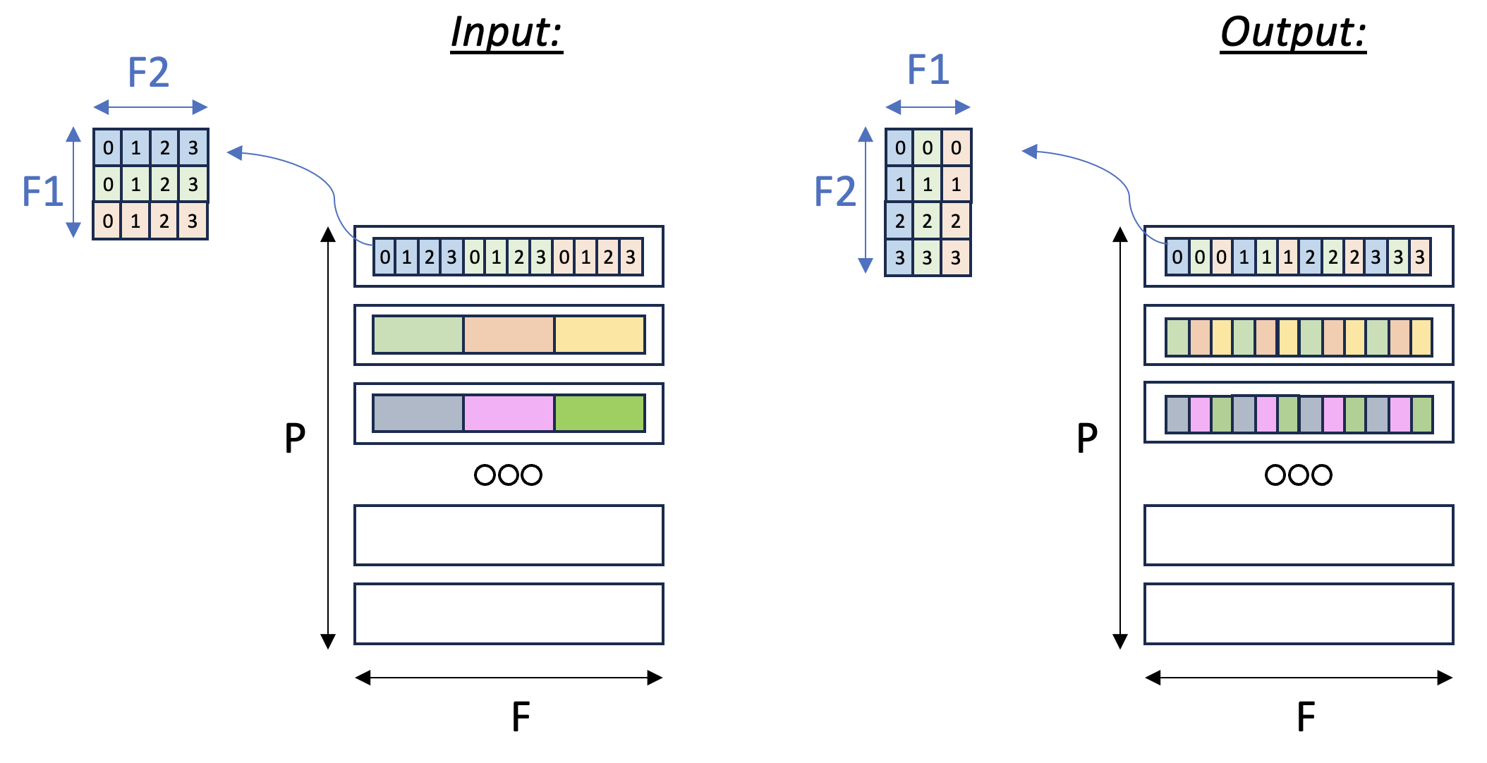
Tensor F1:F2 Transpose
 1import nki
 2import nki.language as nl
 3import nki.isa as nisa
 4
 5
 6@nki.jit
 7def tensor_transpose2D_kernel_(in_tensor, shape2D):
 8  """
 9  NKI kernel to reorder the elements on axis[1] of the input tensor.
10
11  Every row of the input tensor is a flattened row-major 2D matrix.
12  The shape2D argument defines the dimensions of the flattened matrices (#rows,#cols).
13  Our goal in this kernel is to transpose these flattened 2D matrices, i.e. make them (#cols,#rows).
14
15  Example:
16      in_tensor = [a0,a1,a2,a3,b0,b1,b2,b3,c0,c1,c2,c3]
17      shape2D = (3,4)
18  this means that in_tensor has 3 rows and 4 columns, i.e. can be represented as:
19      [a0,a1,a2,a3]
20      [b0,b1,b2,b3]
21      [c0,c1,c2,c3]
22  after transpose, we expect to get:
23      [a0,b0,c0]
24      [a1,b1,c1]
25      [a2,b2,c2]
26      [a3,b3,c3]
27  Thus, out_tensor is expected to be [a0,b0,c0,a1,b1,c1,a2,b2,c2,a3,b3,c3]
28
29  Args:
30    in_tensor: an input tensor
31    shape2D: tuple representing the dimensions to be transposed: (#rows, #cols)
32  """
33  out_tensor = nl.ndarray(in_tensor.shape, dtype=in_tensor.dtype,
34                          buffer=nl.shared_hbm)
35  # Gather input shapes
36  sz_p, _ = in_tensor.shape
37
38  # Load input data from external memory to on-chip memory
39  in_tile = nl.ndarray(in_tensor.shape, dtype=in_tensor.dtype, buffer=nl.sbuf)
40  nisa.dma_copy(dst=in_tile, src=in_tensor)
41
42  # Performing f1/f2 transpose
43  # ==========================
44  # The desired transpose pattern is provided as an input:
45  sz_f1, sz_f2 = shape2D
46
47  # Perform the transposition via element-wise SBUF-to-SBUF copies
48  # with index arithmetic to scatter elements into transposed positions.
49  # RHS traverses an F1 x F2 matrix in row major order
50  # LHS traverses an F2 x F1 (transposed) matrix in row major order
51  out_tile = nl.ndarray(shape=(sz_p, sz_f2*sz_f1), dtype=in_tensor.dtype,
52                        buffer=nl.sbuf)
53  for i_f1 in nl.affine_range(sz_f1):
54    for i_f2 in nl.affine_range(sz_f2):
55      nisa.tensor_copy(dst=out_tile[:, nl.ds(i_f2*sz_f1+i_f1, 1)],
56                       src=in_tile[:, nl.ds(i_f1*sz_f2+i_f2, 1)])
57
58  # Finally, we store out_tile to external memory
59  nisa.dma_copy(dst=out_tensor, src=out_tile)
60
61  return out_tensor
The main concept introduced in this example is a 2D memory access
pattern per partition, via additional indices. We copy in_tile into
out_tile, while traversing the memory in different access patterns
between the source and destination, thus achieving the desired
transposition.
You may download the full runnable script from Transpose2d tutorial.
Case #3 - 2D pooling operation#
Lastly, we examine a case of
dimensionality reduction. We implement a 2D MaxPool operation, which
is used in many vision neural networks. This operation takes
C x [H,W] matrices and reduces each matrix along the H and W
axes. To leverage free-dimension flexible indexing, we can map the C
(parallel) axis to the P dimension and H/W (contraction)
axes to the F dimension.
Performing such a 2D pooling operation requires a 4D memory access
pattern in the F dimension, with reduction along two axes. The figure below illustrates the input and output tensor layouts.
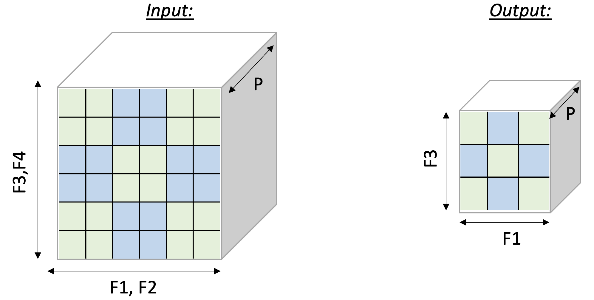
2D-Pooling Operation (reducing on axes F2 and F4)
 1import nki
 2import nki.language as nl
 3
 4@nki.jit
 5def tensor_maxpool_kernel_(in_tensor, sz_pool):
 6  """NKI kernel to compute a 2D max-pool operation
 7
 8  Args:
 9      in_tensor: an input tensor, of dimensions C x H x W
10      sz_pool: integer P representing a (square) pool-window size
11  Returns:
12      out_tensor: the resulting output tensor, of dimensions C x (H/P) x (W/P)
13  """
14
15  # Get input/output dimensions
16  sz_p, sz_hin, sz_win = in_tensor.shape
17  sz_hout, sz_wout = sz_hin // sz_pool, sz_win // sz_pool
18  out_tensor = nl.ndarray((sz_p, sz_hout, sz_wout), dtype=in_tensor.dtype,
19                          buffer=nl.shared_hbm)
20
21  # Load input data from external memory to on-chip memory
22  in_tile = nl.load(in_tensor)
23
24  # Perform the pooling operation using an access pattern to create a 5D view:
25  # [sz_p, sz_hout, sz_wout, sz_pool, sz_pool]
26  # The pool dimensions are placed last so we can reduce over them.
27  pool_view = in_tile.ap([
28    [sz_hin * sz_win, sz_p],      # partition stride
29    [sz_pool * sz_win, sz_hout],   # outer row stride (hop by pool rows)
30    [sz_pool, sz_wout],            # outer col stride (hop by pool cols)
31    [sz_win, sz_pool],             # inner row stride (within pool window)
32    [1, sz_pool],                  # inner col stride (within pool window)
33  ])
34  out_tile = nl.max(pool_view, axis=[3, 4])
35
36  # Store the results back to external memory
37  nl.store(out_tensor, value=out_tile)
38
39  return out_tensor
40
41
42if __name__ == "__main__":
43    import torch
44    import torch_xla
45
46    device = torch_xla.device()
47
48    # Now let's run the kernel
49    POOL_SIZE = 2
50    C, HIN, WIN = 2, 6, 6
51    HOUT, WOUT = HIN//POOL_SIZE, WIN//POOL_SIZE
52
53    in_tensor = torch.arange(C * HIN * WIN, dtype=torch.bfloat16).reshape(C, HIN, WIN).to(device=device)
54    out_tensor = tensor_maxpool_kernel_(in_tensor, POOL_SIZE)
55
56    print(in_tensor, out_tensor) # an implicit XLA barrier/mark-step
This document is relevant for: Trn2, Trn3