This document is relevant for: Inf1, Inf2, Trn1, Trn2, Trn3

Inter-node Collective Communications with AWS Neuron#

This topic explores inter-node collective communication algorithms and optimization strategies for AWS Neuron distributed workloads. It covers the implementation details of Ring, Mesh, and Recursive Doubling-Halving algorithms for coordinating data exchange across multiple nodes connected via EFA (Elastic Fabric Adapter) networks.

Overview#

Inter-node collective communication enables efficient data exchange between NeuronCores distributed across multiple physical nodes in a cluster. This document examines three primary algorithmic approaches: Ring, Mesh, and Recursive Doubling-Halving (RDH), with each optimized for different cluster sizes and message characteristics. The choice of algorithm depends on the trade-offs between step latency (O(N), O(1), O(logN)) and network bandwidth utilization, with performance further influenced by EFA network topology and message size considerations.

Applies to#

This concept is applicable to:

Distributed Training: Collective communication aggregates and synchronizes gradients across workers to maintain model consistency. In this scenario, collective operations enable workers to compute gradient sums across all nodes, ensuring uniform parameter updates.
Distributed Inference: During inference, collective communication distributes requests across multiple accelerators in serving nodes, optimizing resource utilization and maintaining low latency under high loads.

Introduction: About Collectives on Neuron#

Also see Intra-node Collective Communications with AWS Neuron.

Collective Communication Operations#

We define the following denotations:

N: the number of participating ranks in a communication group
C: a “chunk”, which is a piece of data (subset of tensor data transmitted at each algorithm step) with size equaling to that of a rank’s input in AllGather, or output in ReduceScatter
B: the size of both the input and output buffer in AllReduce. In that context, C = B / N

Now we establish the following collective operations:

Table 2 Collective Operations#
Operation Type	Input Size	Output Size	Explanation
AllGather	C	N * C	Each rank starts with a chunk and ends with everyone else’s chunks
ReduceScatter	N * C	C	Each rank starts with N chunks, and ends with a unique chunk which is fully reduced among the N ranks
AllReduce	B = N * C	B = N * C	Each rank contributes B, and ends with B which is fully reduced among the N ranks. AllReduce can be seen as a concatenation of ReduceScatter followed by AllGather
AllToAll	B = N * C	B = N * C	Each rank starts with N chunks, and ends with the N in a way that the pieces of data were transposed between the ranks r0[A0, A1] r1[B0, B1] → r0[A0, B0], r1 [A1, B1]

The execution time of a collective communication operation consists of two parts: step latency + data transfer time. As mentioned above, the per-hop or point-to-point latency is ~15us. On the other hand, the transfer time is a function of the buffer/message size. For example, to transfer 1KiB, 1MiB, and 1GiB at 50Gbps takes 160ns, 160us, and 160ms respectively. Therefore, the collectives communication problem is latency dominant for small sizes, and throughput dominant for large sizes, and a mix for mid-sizes. This requires us to incorporate different strategies and algorithms for each range.

Communication Groups - Only One Rank per Node#

When distributing a ML workload across multiple nodes, communication groups are always formed with symmetry:

The number of participating ranks on each node is consistent
These local ranks must have the same intra-node indices

As the name suggests, one-rank-per-node groups refer to the simple case where we only need to focus on the network communication between peers.

Ring Algorithm#

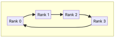
In the Ring algorithm, all participating ranks are joined together in a directed cycle. This algorithm is considered bandwidth optimal, meaning that from each rank’s perspective, it transfers the minimal amount of data. For instance, in the AllGather and ReduceScatter cases we have: number_of_steps * chunk_size = (N - 1) * C.

Ring’s O(N) number of hops means it has linear step latency, making it not suitable for large clusters or the latency-bound small message sizes. However, because each rank only receives from and sends to a fixed peer, the Ring algorithm does not incur any ingress congestion. Furthermore, we can arrange the neighbors in Ring to be topologically close to each other in the substrate network, which reduces the congestion between the global inflight transactions on core switches. As a result, Ring tends to push for the highest bandwidth utilization rate with large message sizes.

Ring AllGather#

In step 0, each rank r sends its input chunk to its downstream peer. In step 1, each rank sends the chunk it just received from the upstream peer further to downstream, and the process repeats until all chunks have traversed the ring.

Ring ReduceScatter#

In step 0, each rank r sends its (r-1)th chunk to its downstream. In step 1, each rank reduces the chunk it just received with the same indexed chunk from its own input, and then sends the result to downstream. This process goes on until each rank has its output chunk fully traversed the ring and reduced among all ranks.

In practice, each ReduceScatter step consists of three components: network receive, local reduction, and network send. To hide the serial latency, an implementation trick is to further break a chunk of data into slices to pipeline the communication and reduction.

Ring AllReduce#

This algorithm is a concatenation of the above two patterns (ReduceScatter followed by AllGather). Its traffic is doubled since we need to traverse the ring twice, but still minimal/optimal.

Mesh Algorithm#

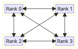
The Mesh algorithm aims to optimize step latency for small message sizes. Rather than transferring data point-to-point like in Ring and accumulating hop latency along the steps. Consequently, there is no extra overhead in Mesh with traffic = number_of_peers * chunk_size = (N - 1) * C.

The mesh communication pattern suffers from ingress congestion because each rank directly receives from all peers. Even small variances in the start time of an operation will cause the fast starters to saturate disproportionately high fractions of the switch and NIC bandwidth, congesting the rest of the transactions by the slower ranks. Furthermore, the fact that one has to communicate with multiple peers means that some of the network paths will be longer (go through higher level of switches) and hence subject to congestion and queuing delays. As a result, Mesh does not scale well to large clusters and/or message sizes.

Mesh AllGather#

It directly broadcasts data from each rank to all the other peers in one step, hence achieving O(1) latency.

Mesh ReduceScatter#

Similarly, Mesh ReduceScatter scatters the input of each rank to the other peers, and then locally reduces the N-1 received chunks, plus the self chunk into the output.

Mesh AllReduce#

This algorithm is a concatenation of the above two patterns (ReduceScatter followed by AllGather). Its traffic is doubled since we need to run Mesh twice, but still minimal/optimal.

Single-step Mesh Algorithm (AllReduce)#

The Single-step Mesh algorithm is a variant of Mesh specifically designed for AllReduce. The goal is to trade off bandwidth optimality for a reduced number of hops (from 2 to 1). Rather than simply concatenating ReduceScatter and AllGather, we can have each rank duplicate and broadcast its whole input buffer to all peers. Upon receiving these duplicates, a rank will reduce the whole buffer to its output. Remember that each hop is expected to add ~15 us latency. Single-step Mesh outperforms regular Mesh for sufficiently small cluster and/or message sizes where the extra data transfer time is shorter than 15 us.

Table 3 Mesh Algorithm Comparison#
Algorithm	# steps	Network Traffic Amount per Rank
Mesh AllGather	1	optimal = (N - 1) * C
Mesh ReduceScatter	1	optimal = (N - 1) * C
Mesh AllReduce	2	optimal = 2 * (N - 1) * C
Single-step Mesh AllReduce	1	not optimal = (N - 1) * N * C

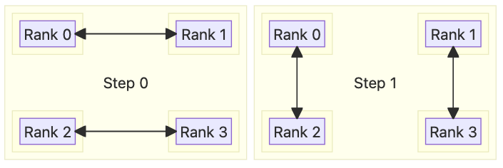
Recursive Doubling and Halving (RDH) Algorithm#

(inspired by https://web.cels.anl.gov/~thakur/papers/ijhpca-coll.pdf)

The Recursive Doubling and Halving (RDH) algorithm works to find the middle ground between Mesh and Ring in both step latency and bandwidth utilization, in a communication group with N = 2^p members.

There is no additional overhead in RDH with traffic = (1 + 2 + 4 ...) * chunk_size = (N - 1) * C. Corresponding to the number of steps, the step latency of RDH is O(logN) or O(p). In respect to congestion deficiency, having log(N) peers poses ingress contentions, but in the implementation, we can issue send/receive credits with rate control to mitigate such issues. Effectively, a rank will only talk to one single peer at any given time, resulting in several steady streams of high-speed transfer and a relatively high amortized bandwidth utilization. Overall, RDH is suitable for large clusters with medium/large sized messages.

When representing the indices in binary, they are obtained by flipping each of the p bits of the current rank’s index.

Recursive-Doubling AllGather#

It works by having each rank sequentially communicating with log(N) peers. In each step of AllGather, a rank sends all the chunks it has collected so far, and receives the equal amount of new chunks from its peer, hence doubling the amount of data. The algorithm follows a classic Recursive-Doubling communication style.

Recursive-Halving ReduceScatter#

This algorithm works similarly — in each step, a rank sends half of the partially reduced chunks so far to its peer, and receives the other peer’s half of partial chunks. It then reduces the self chunks and the received chunks together, and we repeat the process with the problem space exactly halved.

Recursive-Halving AllReduce#

Again, AllReduce works by concatenating ReduceScatter and AllGather.

Algorithm Summary#

Table 4 Algorithm Comparison#
Algorithm	Step Latency	Network BW Utilization	Suitable Group Sizes	Suitable Message Sizes
Ring	O(N)	High	Small-to-medium	Large
Mesh	O(1)	Low	Small	Small
RDH	O(logN)	> Mesh; < Ring	Medium-to-large	Small-to-medium

Communication Groups - Multiple Ranks per Node#

Orchestrating collective communication operations across distributed computing systems presents a fundamental challenge when multiple processing ranks are deployed per node. The complexity arises from the need to efficiently coordinate data exchange both within individual nodes (intra-node) and across the network between different nodes (inter-node), each with distinct bandwidth characteristics, latency profiles, and optimal communication patterns.

Traditional flat communication algorithms that treat all ranks uniformly often fail to exploit the inherent hierarchical structure of modern distributed systems, leading to suboptimal performance and scalability bottlenecks.

Hierarchical algorithms address this challenge by recognizing and leveraging the two-tier nature of distributed systems, strategically decomposing global operations into separate intra-node and inter-node phases that can each be optimized independently while maintaining overall correctness and efficiency.

Hierarchical Algorithm#

The Hierarchical algorithm is a powerful framework to break down a multiple-rank-per-node operation into stages of pure intra-node and inter-node communication.

The hierarchical algorithm implementation employs a plug-and-play mechanism to allow for any combination of intra-node and inter-node algorithms — and we simply choose the most optimal one for each communication stage.

The latency and throughput properties of the Hierarchical algorithm is therefore dependent on the selected sub-algorithms. However, it’s worth calling out that by breaking a global communication into intra-node and inter-node dimensions, we promote the principle of divide and conquer and it matters especially to the total latency. For example by choosing Ring + Ring, the latency is O(X) + O(Y), where X is the number of nodes and Y intra-node ranks. That is significantly better than Flat Ring’s O(X * Y).

Overall, the Hierarchical algorithm is versatile to work well across a wide range of group and message sizes. For example, small groups + sizes can go to intra-node Mesh + inter-node Mesh, and large groups + sizes can go to intra-node KangaRing + inter-node RDH.

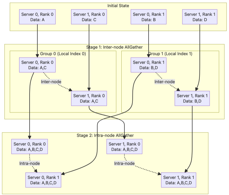
Global AllGather = inter-node AllGather + intra-node AllGather#

Let’s assume there are X servers globally, each containing Y ranks. The first step of the hierarchical algorithm is to form Y rank lists where each contains X ranks who have the same local index. Later, we run AllGather on these inter-node groups in parallel and each rank ends up with X chunks. Finally, we form X rank lists each of all the Y ranks on one node, and run intra-node AllGather again to further broadcast the data. By the end, everyone has all the (X * Y) chunks.

Because the inter EFA interface has lower bandwidth than that of the intra-node interface, and that the first stage incurs less traffic than the second, we choose to run the inter-node communication first.

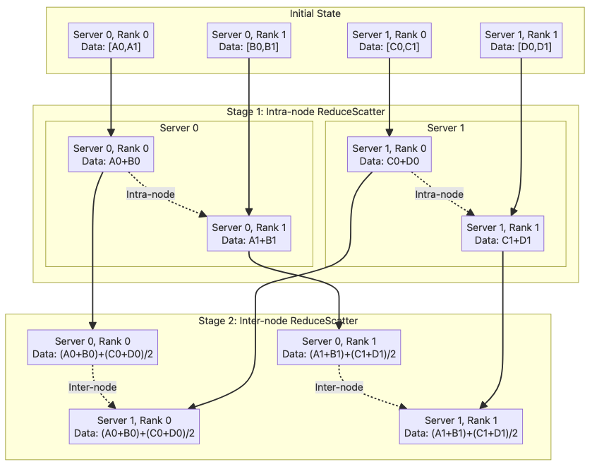
Global ReduceScatter = intra-node ReduceScatter + inter-node ReduceScatter#

We can run intra-node ReduceScatter first on X parallel rank lists of Y local ranks, reducing the buffer size to 1/Y of the original size. Notice that each rank will end up holding a different 1/Y corresponds to its local index. Next, we run inter-node ReduceScatter on Y parallel rank lists of X network ranks, further reducing the buffer on each global rank a unique 1/(X * Y) chunk of the original.

The order of the intra- and inter-node stages is flipped when compared to AllGather, because now the second stage has less traffic.

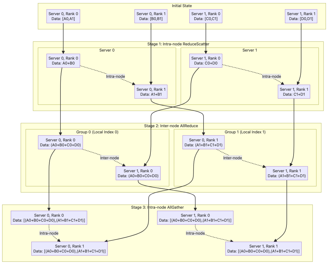
Global AllReduce = intra-node ReduceScatter + inter-node AllReduce + intra-node AllGather#

We first run an intra-node ReduceScatter to break down the buffer size to 1/Y of the original. Then we run an inter-node AllReduce. Again, each inter-node group will work on a different 1/Y section of the original buffer, so there’s no duplicated work. And lastly, we run an intra-node AllGather to broadcast the whole buffer to everyone.

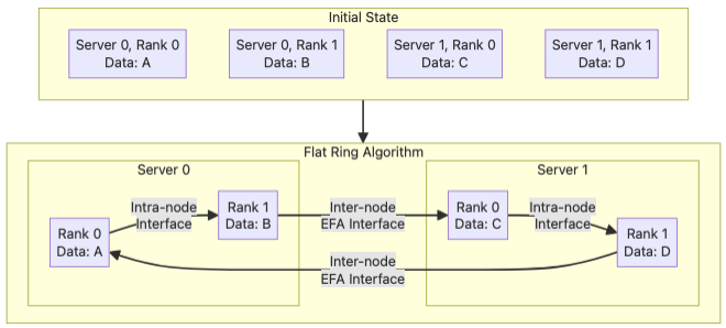
Flat Ring Algorithm (Edge cases only)#

The Flat Ring algorithm works by connecting all the global ranks in a directed cycle. Ranks local to a single server are connected in an open chain with the intra-node communication interface, and the two ends will be joined to chains on other servers with the inter-node EFA interface.

The step latency is O(X * Y) - X is the number of nodes and Y intra-node ranks - and the network bandwidth utilization is high. However, one caveat is that each EFA interface is connected to a different Trainium Chip. So, to utilize all of them, we need to run multiple directed cycles (called channels) in parallel, thus reducing the transfer size and efficiency of each cycle, besides causing high context switching overheads in the collective execution cores. We only enable Flat Ring on Trn1 for large message size cases where it has a clear edge.

More information#