This document is relevant for: Trn1, Trn2

How to debug models in PyTorch NeuronX#

Torch-XLA evaluates operations lazily, which means it builds a symbolic graph in the background and the graph is executed in hardware only when the users request (print) for the output or a mark_step is encountered. To effectively debug training scripts with torch-xla, please use one of the approaches mentioned below:

Printing metrics#

Torch-xla provides a utility that records metrics of different sections of the code. These metrics can help figure out things like: How much time is spent in compilation? How much time is spent in execution? To check the metrics:

Import metrics: import torch_xla.debug.metrics as met
Print metrics at the end of the step: print(met.metrics_report())

Printing metrics should produce an output that looks like this:

Metric: CompileTime
  TotalSamples: 1
  Accumulator: 09s969ms486.408us
  Percentiles: 1%=09s969ms486.408us; 5%=09s969ms486.408us; 10%=09s969ms486.408us; 20%=09s969ms486.408us; 50%=09s969ms486.408us; 80%=09s969ms486.408us; 90%=09s969ms486.408us; 95%=09s969ms486.408us; 99%=09s969ms486.408us
.....
Metric: ExecuteTime
  TotalSamples: 1
  Accumulator: 186ms062.970us
  Percentiles: 1%=186ms062.970us; 5%=186ms062.970us; 10%=186ms062.970us; 20%=186ms062.970us; 50%=186ms062.970us; 80%=186ms062.970us; 90%=186ms062.970us; 95%=186ms062.970us; 99%=186ms062.970us
....
Metric: TensorsGraphSize
  TotalSamples: 1
  Accumulator: 9.00
  Percentiles: 1%=9.00; 5%=9.00; 10%=9.00; 20%=9.00; 50%=9.00; 80%=9.00; 90%=9.00; 95%=9.00; 99%=9.00
Metric: TransferFromServerTime
  TotalSamples: 2
  Accumulator: 010ms130.597us
  ValueRate: 549ms937.108us / second
  Rate: 108.372 / second
  Percentiles: 1%=004ms948.602us; 5%=004ms948.602us; 10%=004ms948.602us; 20%=004ms948.602us; 50%=006ms181.995us; 80%=006ms181.995us; 90%=006ms181.995us; 95%=006ms181.995us; 99%=006ms181.995us
Metric: TransferToServerTime
  TotalSamples: 6
  Accumulator: 061ms698.791us
  ValueRate: 007ms731.182us / second
  Rate: 0.665369 / second
  Percentiles: 1%=006ms848.579us; 5%=006ms848.579us; 10%=006ms848.579us; 20%=007ms129.666us; 50%=008ms940.718us; 80%=008ms496.166us; 90%=024ms636.413us; 95%=024ms636.413us; 99%=024ms636.413us
Metric: TransferToServerTransformTime
  TotalSamples: 6
  Accumulator: 011ms835.717us
  ValueRate: 001ms200.844us / second
  Rate: 0.664936 / second
  Percentiles: 1%=108.403us; 5%=108.403us; 10%=108.403us; 20%=115.676us; 50%=167.399us; 80%=516.659us; 90%=010ms790.400us; 95%=010ms790.400us; 99%=010ms790.400us
.....
Counter: xla::_copy_from
  Value: 7
Counter: xla::addmm
  Value: 2
Counter: xla::empty
  Value: 5
Counter: xla::t
  Value: 2
....
Metric: XrtCompile
  TotalSamples: 1
  Accumulator: 09s946ms607.609us
  Mean: 09s946ms607.609us
  StdDev: 000.000us
  Percentiles: 25%=09s946ms607.609us; 50%=09s946ms607.609us; 80%=09s946ms607.609us; 90%=09s946ms607.609us; 95%=09s946ms607.609us; 99%=09s946ms607.609us
Metric: XrtExecute
  TotalSamples: 1
  Accumulator: 176ms932.067us
  Mean: 176ms932.067us
  StdDev: 000.000us
  Percentiles: 25%=176ms932.067us; 50%=176ms932.067us; 80%=176ms932.067us; 90%=176ms932.067us; 95%=176ms932.067us; 99%=176ms932.067us
Metric: XrtReadLiteral
  TotalSamples: 2
  Accumulator: 608.578us
  Mean: 304.289us
  StdDev: 067.464us
  Rate: 106.899 / second
  Percentiles: 25%=236.825us; 50%=371.753us; 80%=371.753us; 90%=371.753us; 95%=371.753us; 99%=371.753us

As seen, you can get useful information about graph compile times/execution times. You can also know which operators are present in the graph, which operators are run on the CPU and which operators are run on an XLA device. For example, operators that have a prefix aten:: would run on the CPU, since they do not have xla lowering. All operators with prefix xla:: would run on an XLA device. Note: aten operators that do not have xla lowering would result in a graph fragmentation and might end up slowing down the entire execution. If you encounter such operators, create a request for operator support.

Printing tensors#

Users can print tensors in their script as below:

import os
import torch
import torch_xla
import torch_xla.core.xla_model as xm

device = xm.xla_device()
input1 = torch.randn(2,10).to(device)
# Defining 2 linear layers
linear1 = torch.nn.Linear(10,30).to(device)
linear2 = torch.nn.Linear(30,20).to(device)

# Running forward
output1 = linear1(input1)
output2 = linear2(output1)
print(output2)

Since torch-xla evaluates operations lazily, when you try to print output2 , the graph associated with the tensor would be evaluated. When a graph is evaluated, it is first compiled for the device and executed on the selected device. Note: Each tensor would have a graph associated with it and can result in graph compilations and executions. For example, in the above script, if you try to print output1 , a new graph is cut and you would see another evaluation. To avoid multiple evaluations, you can make use of mark_step (next section).

Use mark_step#

Torch-XLA provides an api called mark_step which evaluates a graph collected up to that point. While this is similar to printing of an output tensor wherein a graph is also evaluated, there is a difference. When an output tensor is printed, only the graph associated with that specific tensor is evaluated, whereas mark_step enables all the output tensors up to mark_step call to be evaluated in a single graph. Hence, any tensor print after mark_step would be effectively free of cost as the tensor values are already evaluated. Consider the example below:

import os
import torch
import torch_xla
import torch_xla.core.xla_model as xm
import torch_xla.debug.metrics as met

device = xm.xla_device()
input1 = torch.randn(2,10).to(device)
# Defining 2 linear layers
linear1 = torch.nn.Linear(10,30).to(device)
linear2 = torch.nn.Linear(30,20).to(device)

# Running forward
output1 = linear1(input1)
output2 = linear2(output1)
xm.mark_step()
print(output2)
print(output1)
# Printing the metrics to check if compilation and execution occurred
print(met.metrics_report())

In the printed metrics, the number of compiles and executions is only 1, even though 2 tensors are printed. Hence, to avoid multiple graph evaluations, it is recommended that you visualize tensors after a mark_step . You can also make use of the add_step_closure api for this purpose. With this api, you pass in the tensors that needs to be visualized/printed. The added tensors would then be preserved in the graph and can be printed as part of the callback function passed to the api. Here is a sample usage: pytorch/xla

Note: Graph compilations can take time as the compiler optimizes the graph to run on device.

Using Eager Debug Mode#

Eager debug mode provides a convenient utility to step through the code and evaluate operators one by one for correctness. Eager debug mode is useful to inspect your models the way you would do in eager-mode frameworks like PyTorch and Tensorflow. With Eager Debug Mode operations are executed eagerly. As soon as an operation is registered with torch-xla, it would be sent for compilation and execution. Since compiling a single operation, the time spent would be minimal. Moreover, the chances of hitting the framework compilation cache increases as models would have repeated operations throughout. Consider example 1 below:

# Example 1

import os
# You need to set this env variable before importing torch-xla
# to run in eager debug mode.
os.environ["NEURON_USE_EAGER_DEBUG_MODE"] = "1"

import torch
import torch_xla
import torch_xla.core.xla_model as xm
import torch_xla.debug.metrics as met

device = xm.xla_device()
input1 = torch.randn(2,10).to(device)
# Defining 2 linear layers
linear1 = torch.nn.Linear(10,30).to(device)
linear2 = torch.nn.Linear(30,20).to(device)

# Running forward
output1 = linear1(input1)
output2 = linear2(output1)

# Printing the metrics to check if compilation and execution occurred
# Here, in the metrics you should notice that the XRTCompile and XRTExecute
# value is non-zero, even though no tensor is printed. This is because, each
# operation is executed eagerly.
print(met.metrics_report())

print(output2)
print(output1)
# Printing the metrics to check if compilation and execution occurred.
# Here the XRTCompile count should be same as the previous count.
# In other words, printing tensors did not incur any extra compile
# and execution of the graph
print(met.metrics_report())

As seen from the above scripts, each operator is evaluated eagerly and there is no extra compilation when output tensors are printed. Moreover, together with the on-disk Neuron persistent cache, eager debug mode only incurs one time compilation cost when the ops is first run. When the script is run again, the compiled ops will be pulled from the persistent cache. Any changes you make to the training script would result in the re-compilation of only the newly inserted operations. This is because each operation is compiled independently. Consider example 2 below:

# Example 2

import os
# You need to set this env variable before importing torch-xla
# to run in eager debug mode.
os.environ["NEURON_USE_EAGER_DEBUG_MODE"] = "1"

import torch
import torch_xla
import torch_xla.core.xla_model as xm
import torch_xla.debug.metrics as met

os.environ['NEURON_CC_FLAGS'] = "--log_level=INFO"

device = xm.xla_device()
input1 = torch.randn(2,10).to(device)
# Defining 2 linear layers
linear1 = torch.nn.Linear(10,30).to(device)
linear2 = torch.nn.Linear(30,20).to(device)
linear3 = torch.nn.Linear(20,30).to(device)
linear4 = torch.nn.Linear(30,20).to(device)

# Running forward
output1 = linear1(input1)
output2 = linear2(output1)
output3 = linear3(output2)

# Note the number of compiles at this point and compare
# with the compiles in the next metrics print
print(met.metrics_report())

output4 = linear4(output3)
print(met.metrics_report())

Running the above example 2 script after running example 1 script, you may notice that from the start until the statement output2 = linear2(output1) , all the graphs would hit the persistent cache. Executing the line output3 = linear3(output2) would result in a new compilation for linear3 layer only because the layer configuration is new. Now, when we run output4 = linear4(output3) , you would observe no new compilation happens. This is because the graph for linear4 is same as the graph for linear2 and hence the compiled graph for linear2 is reused for linear4 by the framework’s internal cache.

Eager debug mode avoids the wait times involved with tensor printing because of larger graph compilation. It is designed only for debugging purposes, so when the training script is ready, please remove the NEURON_USE_EAGER_DEBUG_MODE environment variable from the script in order to obtain optimal performance.

By default, in eager debug mode the logging level in the Neuron compiler is set to error mode. Hence, no logs would be generated unless there is an error. Before your first print, if there are many operations that needs to be compiled, there might be a small delay. In case you want to check the logs, switch on the INFO logs for compiler using:

os.environ["NEURON_CC_FLAGS"] = "--log_level=INFO"

Profiling model run#

Profiling model run can help to identify different bottlenecks and resolve issues faster. You can profile different sections of the code to see which block is the slowest. To profile model run, you can follow the steps below:

Add: import torch_xla.debug.profiler as xp
Start server. This can be done by adding the following line after creating xla device: server = xp.start_server(9012)
In a separate terminal, start tensorboard. The logdir should be in the same directory from which you run the script.

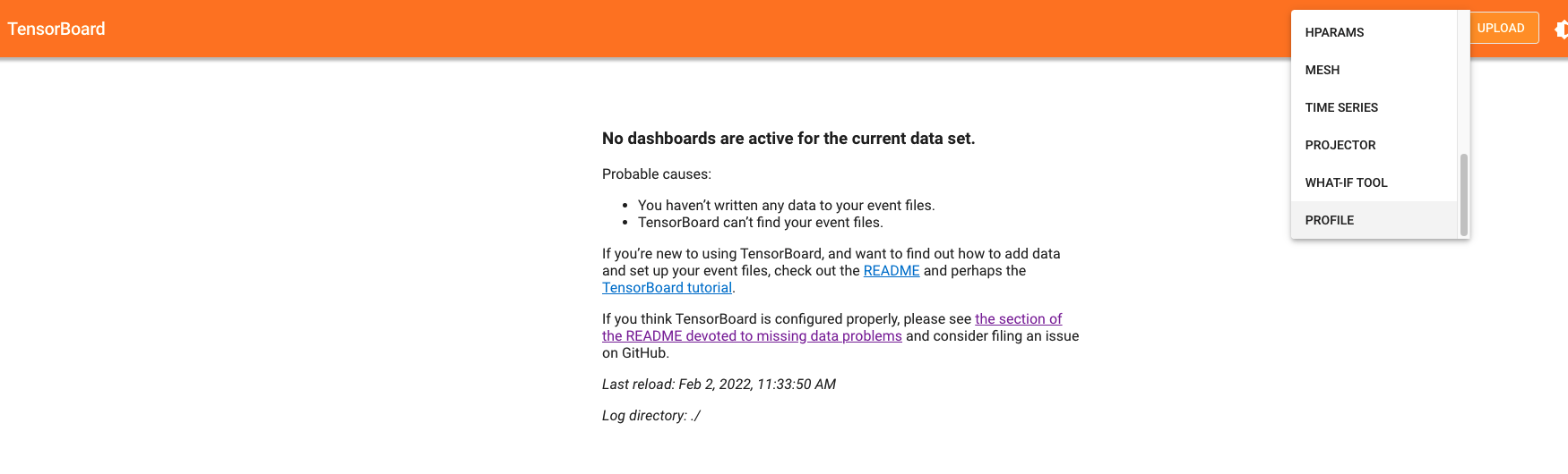
Open the tensorboard on a browser. Go to profile section in the top right. Note: you may have to install the profile plugin using: pip install tensorboard-plugin-profile
When you click on the profile, it should give an option to capture profile. Clicking on capture profile produces the following pop-up.

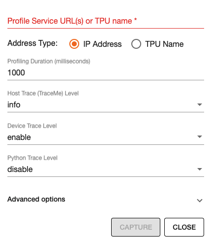
In the URL enter: localhost:9012 . Port in this URL should be same as the one you gave when starting the server in the script.
Once done, click capture and it should automatically load the following page:
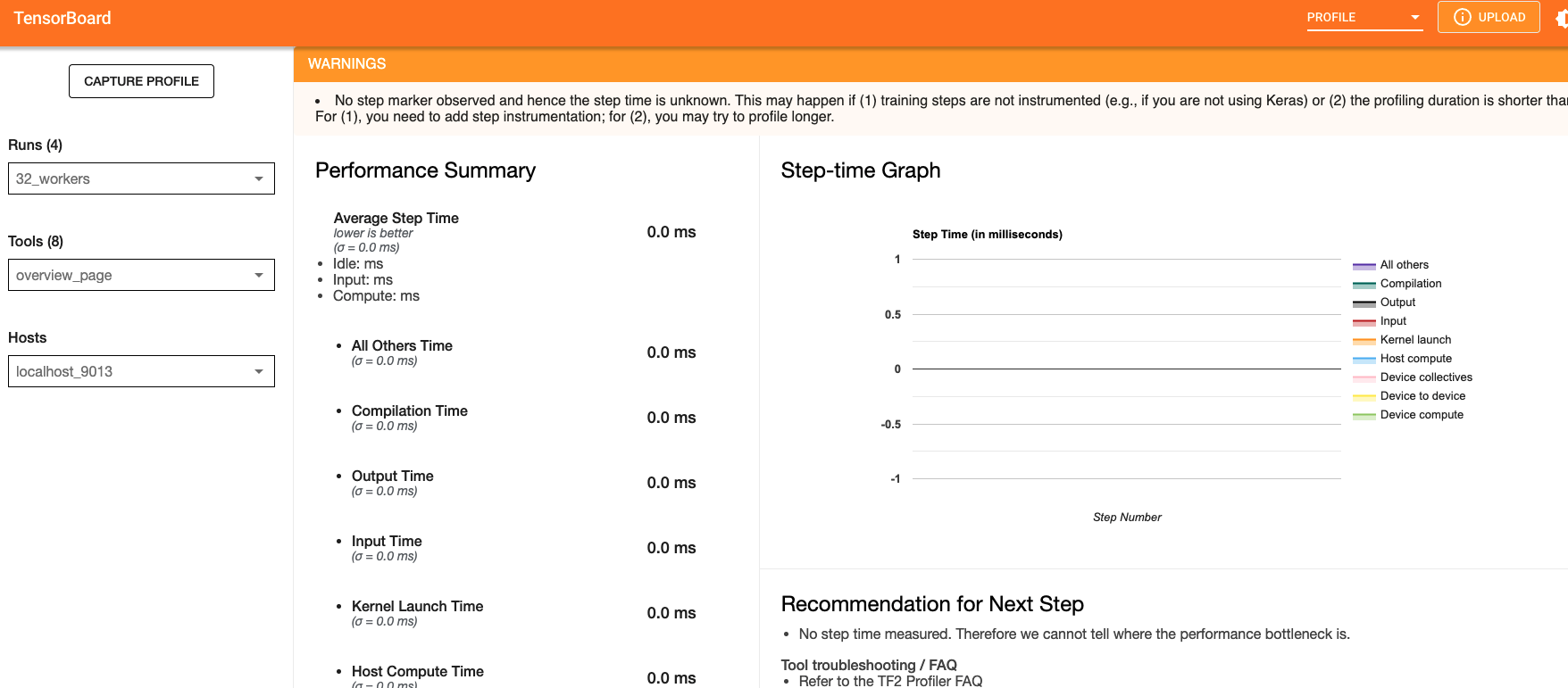
To check the profile for different blocks of code, head to trace_viewer under Tools (on the left column).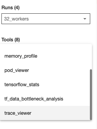
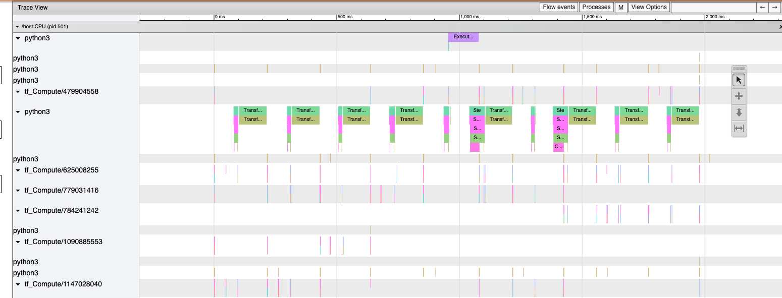
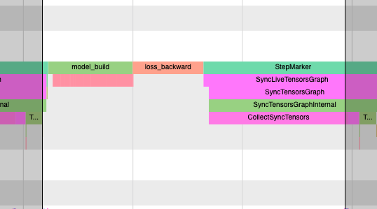
It should show a profile that looks like this:

Note: By default, torch-xla would time different blocks of code inside the library. However, you can also profile block of code in your scripts. This can be done by adding the code within a xp.Trace context as follows:

....
for epoch in range(total_epochs):
    inputs = torch.randn(1,10).to(device)
    labels = torch.tensor([1]).to(device)
    with xp.Trace("model_build"):
        loss = model(inputs, labels)
    with xp.Trace("loss_backward"):
        loss.backward()
....

It should produce a profile that has the model_build and loss_backward section timed. This way you can time any block of script for debugging.

Note: If you are running your training script in a docker container, to view the tensorboard, you should launch the docker container using flag: --network host eg. docker run --network host my_image:my_tag

Snapshotting With Torch-Neuronx 2.1#

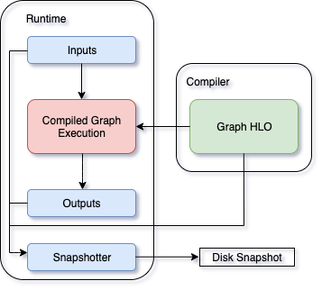
Snapshotting models can be used to dump debug information that can then be sent to the Neuron team. Neuron execution relies on a series of compiled graphs. Internally, graph HLOs are used as an intermediate representation which is then compiled. Then, during execution, the graph inputs are passed to the Neuron runtime, which produces outputs using the compiled graph. Snapshotting saves the inputs to a graph execution, executes the graphs, saves the outputs of the execution, and then bundles and dumps the inputs, outputs and graph HLO in one file. This is illustrated here:

This feature can be enabled using the following environment variables, which can be set at the beginning of your script as follows (./dump is the snapshot dump directory that will be created):

....
os.environ["XLA_FLAGS"] = "--xla_dump_hlo_snapshots --xla_dump_to=./dump"
....

This environment variable will produce snapshots in the ./dump folder with the extension .decomposed_hlo_snapshot at every iteration for every process. For example, files that look like the following would be produced.

SyncTensorsGraph.27737-process000000-executable000003-device000000-execution000496.inputs.decomposed_hlo_snapshot

Note that NEURON_FRAMEWORK_DEBUG does not need to be set, as in torch-neuronx 1.13. Also note that NEURON_DUMP_HLO_SNAPSHOT and NEURON_NC0_ONLY_SNAPSHOT environment variables used in torch-neuronx 1.13 are now no longer used to control snapshot dumping.

Snapshots can take up a large amount of disk space. To avoid running out of disk space, you can limit the snapshoting for a certain rank, such as rank 0. The following example code would work with torchrun utility which sets the RANK environment variable for each process:

if os.environ.get("RANK", "0") == "0":
    os.environ["XLA_FLAGS"]="--xla_dump_hlo_snapshots --xla_dump_to=./dump"

or if not using torchrun:

import torch_xla.core.xla_model as xm

....
if xm.is_master_ordinal():
    os.environ["XLA_FLAGS"]="--xla_dump_hlo_snapshots --xla_dump_to=./dump"
....

Torch-NeuronX 2.1+ provides a register_hlo_snapshot_callback API to allow more control over when to dump the snapshot. By default, Torch-NeuronX 2.1+ includes the following callback function:

def _dump_hlo_snapshot_callback(name: str, addressable_device_index: int, execution_count: int) -> str:
    return 'inputs'

As the return value is always ‘inputs’, the backend will always dump snapshot files containing HLO and input data only. Recognized return value keywords are ‘inputs’ and ‘outputs’. If the return value is an empty string ‘’, then the backend will skip this dump. If the return value is ‘inputs outputs’, then the backend will dump two snapshot files for each execution, one holding inputs, and another one holding outputs.

To implement selective dumping, we can make use of the callback function’s parameters name, addressable_device_index, execution_count , where:

name is a string that stands for the HLO graph’s name.
addressable_device_index is an integer that refers to the index of the addressable Neuron device as one NEFF can load onto multiple addressable Neuron devices (NeuronCores) for SPMD executions. Note that this is not the same as the worker process rank in multi-process execution, in which RANK/xm.get_ordinal() or LOCAL_RANK/xm.get_local_ordinal() should be used. See examples above.
execution_count is an integer that indicates the value of an internal execution counter that increments by one for each execution of a compiled graph when HloSnapshot dumping is requested. Note that each compiled graph maintains multiple execution counters, one for each addressable device that it loads onto.

For example, the following will dump snapshot files containing outputs at execution #2 (Note that this is graph execution number, not the iteration or step; for iteration or step, see the next example):

def callback(name, addressable_device_index, execution_count):
    if execution_count == 2:
        return 'outputs'
    else:
        return ''

import libneuronxla
old_callback = libneuronxla.register_hlo_snapshot_callback(callback)

Callback functions can be use to dump at a certain condition, such as when the global step count equal a value:

step = 0
def callback(name, addressable_device_index, execution_count):
    if step == 5:
        return 'inputs'
    else:
        return ''

import libneuronxla
old_callback = libneuronxla.register_hlo_snapshot_callback(callback)

...
for epoch in range(EPOCHS):
    for idx, (train_x, train_label) in enumerate(train_loader):
        step += 1
...

Note

Snapshot dumping triggered by a runtime error such as NaN is not yet available. It will be available in a feature release.

Snapshotting with Torch-Neuronx 1.13#

Note

If you are using Torch-NeuronX 2.1, please see Snapshotting With Torch-Neuronx 2.1

With Torch-Neuronx 1.13, the snapshotting feature can be enabled using the following environment variables, which can be set at the beginning of your script as follows.

....
os.environ["XLA_FLAGS"] = " --xla_dump_to=dump"
os.environ["NEURON_FRAMEWORK_DEBUG"] = "1"
os.environ["NEURON_DUMP_HLO_SNAPSHOT"] = "1"
....

This set of environment variables will produce snapshots under the dump folder with the extensions .hlo.snapshot.pb or .decomposed_hlo_snapshot at every iteration. For example a file that looks like the following would be produced.

dump/module_SyncTensorsGraph.387.pid_12643.execution_7496.hlo_snapshot.pb

The dumping environment variable can be set and unset at specific iterations as shown in the following example.

....
for step in range(STEPS):
    if step == 20:
        os.environ["NEURON_DUMP_HLO_SNAPSHOT"] = "1"
    else:
        os.environ.pop('NEURON_DUMP_HLO_SNAPSHOT', None)
    train_x = torch.randn(BATCH_SIZE, 28, 28)
    train_x = train_x.to(device)
    loss = model(train_x)
    loss.backward()
    optimizer.step()
    xm.mark_step()
....

Additionally, we provide capabilities to snapshot graphs automatically. The environment variables above can be set as follows:

....
os.environ["XLA_FLAGS"] = " --xla_dump_to=dump"
os.environ["NEURON_FRAMEWORK_DEBUG"] = "1"
os.environ["NEURON_DUMP_HLO_SNAPSHOT"] = "ON_NRT_ERROR"
....

When unexpected errors such as a graph execution producing NaNs occurs, snapshots will be automatically produced and execution will be terminated. Occasionally, for larger models, automatic snapshotting may not capture snapshots due to the device memory being exhausted. In this case, the above flag can be set to os.environ["NEURON_DUMP_HLO_SNAPSHOT"] = "ON_NRT_ERROR_HYBRID", this will allocate memory for inputs on both the device and host memory. In some additional cases, this may still go out of memory and may need to be set to os.environ["NEURON_DUMP_HLO_SNAPSHOT"] = "ON_NRT_ERROR_CPU" to avoid allocating any memory on the device at all for automatic snapshotting.

Snapshot FAQs:#

When should I use this features?

This feature should be used when debugging errors that requires interfacing with and providing debug data to the Neuron team. Snapshotting may be redundant and unnecessary in some situations. For example, when only the model weights are necessary for debugging, methods such as checkpointing may be more convenient to use.

What sort of data is captured with these snapshots?

The type of data captured by these snapshots may include model graphs in HLO form, weights/parameters, optimizer states, intermediate tensors and gradients. This data may be considered sensitive and this should be taken into account before sending the data to the Neuron team.

What is the size of these snapshots?

The size of snapshots can be significant for larger models such as GPT or BERT with several GBs worth of data for larger graphs, so it is recommended to check that sufficient disk space exists before using snapshotting. In addition, limiting the amount of snapshots taken in a run will help to preserve disk space.

Will snapshotting add overhead to my execution?

Snapshotting does add a small overhead to the execution in most cases. This overhead can be significant if snapshots are dumped at every iteration. In order to alleviate some of this overhead, in the case that snapshotting is not necessary on all cores the following environment variable can be set to collect snapshots only on the first core in torch-neuronx 1.13:

....
os.environ["NEURON_NC0_ONLY_SNAPSHOT"] = "1"
....

In torch-neuronx 2.1, use RANK environmental variable when using torchrun or xm.is_master_ordinal() to limit dumping to the first process (see above):

....
if os.environ.get("RANK", "0") == "0":
    os.environ["XLA_FLAGS"]="--xla_dump_hlo_snapshots --xla_dump_to=./dump"
....

or (not using torchrun):

import torch_xla.core.xla_model as xm

....
if xm.is_master_ordinal():
    os.environ["XLA_FLAGS"]="--xla_dump_hlo_snapshots --xla_dump_to=./dump"
....

In addition, checkpointing in tandem with snapshotting can be useful to reduce overhead. A checkpoint close to the problem iteration can be captured, then execution resumed with snapshots enabled.

How can I share snapshots with the Neuron team?

These snapshots can be shared with the Neuron team via S3 bucket.

This document is relevant for: Trn1, Trn2

How to debug models in PyTorch NeuronX

Contents

How to debug models in PyTorch NeuronX#