This document is relevant for: Inf1, Inf2, Trn1, Trn2, Trn3

Profiling a vLLM Inference Workload on AWS Trainium

This tutorial outlines the steps involved in using Neuron Explorer to capture and view system-level and device-level profiles for a vLLM-hosted inference workload on AWS Trainium.

Overview

By following this tutorial you will learn how to:

• Launch a vLLM-hosted inference workload on AWS Trainium with system and device-level profiling enabled

• View the system-level profile using Perfetto

• Identify regions within the system profile that show LLM context-encoding (prefill) and token generation (decode) running on the NeuronDevices, along with the names of the associated compute graphs

• View the device-level profiles for context-encoding & token generation compute graphs in the Neuron Explorer UI

Prepare your environment

The following steps show how to launch a Trainium EC2 instance using the latest Neuron Deep Learning AMI (DLAMI) and then install vLLM so that an example vLLM-hosted model can be profiled using the Neuron Explorer. If you would prefer to use a containerized environment (Docker, EKS), please refer to the Neuron documentation to get started with a Neuron Deep Learning Container (DLC) image that has vLLM pre-installed.

1. Launch a Trainium instance (trn1.32xlarge, trn2.3xlarge, trn2.48xlarge)

   1. Option 1: Launch the instance using the latest AWS Deep Learning AMI (DLAMI), which includes the Neuron SDK preinstalled. Once the instance is launched, please SSH into it and use the virtual environment for neuronx-distributed-inference by following this command -

      1. source /opt/aws_neuronx_venv_pytorch_2_8_nxd_inference/bin/activate

   2. Option 2: If using a fresh Linux instance, manually install the latest Neuron packages by following the AWS Neuron installation guide.

2. Install vLLM

   1. Refer to the Neuron documentation which outlines how to install the Neuron vLLM fork from source.

Step 1: Save a smaller version of your model

When profiling LLMs it is usually desirable to use only a subset of the model’s layers in order to understand model performance and to identify possible bottlenecks. Capturing traces for the entire model could lead to an excessive volume of profiling data, making analysis cumbersome. To address this, the following script takes the Qwen3-8B-base model, truncates it to the first 4 layers, and saves the resulting smaller model for profiling purposes.

import transformers

model_id = "Qwen/Qwen3-8B-Base"
config = transformers.AutoConfig.from_pretrained(model_id)
config.num_hidden_layers = 4
tokenizer = transformers.AutoTokenizer.from_pretrained(model_id)
output_dir = "4layer_qwen3"

model = transformers.AutoModelForCausalLM.from_pretrained(model_id, config=config)
model.save_pretrained(output_dir)
tokenizer.save_pretrained(output_dir)

Save the above python script as save_4layer_qwen.py and then run it using the python interpreter:

python3 ./save_4layer_qwen.py

Once the script has completed, you should see the new 4layer_qwen directory which contains the truncated model.

Step 2: Run a vLLM offline inference workload with profiling enabled

In this step, you will run a small vLLM offline inference script that will compile, run, and profile your 4-layer Qwen3 model on the Trainium chips.

Begin by saving the following python script as qwen3_offline_inference.py:

import os
os.environ['VLLM_NEURON_FRAMEWORK'] = "neuronx-distributed-inference"

# Enable Neuron profiling via environment variables
os.environ['XLA_IR_DEBUG'] = "1"
os.environ['XLA_HLO_DEBUG'] = "1"
os.environ['NEURON_FRAMEWORK_DEBUG'] = "1"
os.environ['NEURON_RT_INSPECT_ENABLE'] = "1"
os.environ['NEURON_RT_INSPECT_SYSTEM_PROFILE'] = "1"
os.environ['NEURON_RT_INSPECT_DEVICE_PROFILE'] = "1"
os.environ['NEURON_RT_INSPECT_OUTPUT_DIR'] = "./neuron_profiles"

from vllm import LLM, SamplingParams

# Sample prompts.
prompts = [
    "The president of the United States is",
    "The capital of France is",
    "The future of AI is",
]
# Create a sampling params object.
sampling_params = SamplingParams(top_k=1)

# Create an LLM instance using the 4-layer Qwen3 model
llm = LLM(
    model="4layer_qwen3",
    max_num_seqs=4,
    max_model_len=128,
    override_neuron_config={
        "enable_bucketing":False,
    },
    device="neuron",
    tensor_parallel_size=8)

# Run inference using the sample prompts
outputs = llm.generate(prompts, sampling_params)

Next, run the offline inference script with a Python interpreter:

python3 ./qwen3_offline_inference.py

After ~60s the script should complete, and you will see a new neuron_profiles directory which contains both system-level and device-level profile traces for this example inference workload.

Step 3: Visualize the system profile for your model

Note

System profiles are currently viewed using the open-source Perfetto tool. Viewing of system profiles will be natively supported by the Neuron Explorer UI in an upcoming release.

Run the following command to generate a Perfetto compatible file from the system profile traces that you previously captured:

neuron-profile view -d ./neuron_profiles --ignore-device-profile \
  --output-format perfetto

The above command generates a file called system_profile.pftrace in your working directory.

Copy the system_profile.pftrace file to your local machine and open up the Perfetto UI in your local web browser.

In the left-hand menu, choose “Open trace file” and select your system_profile.pftrace file to view the system profile. Expand the first row under Default Workspace and you will see a timeline view similar to the following:

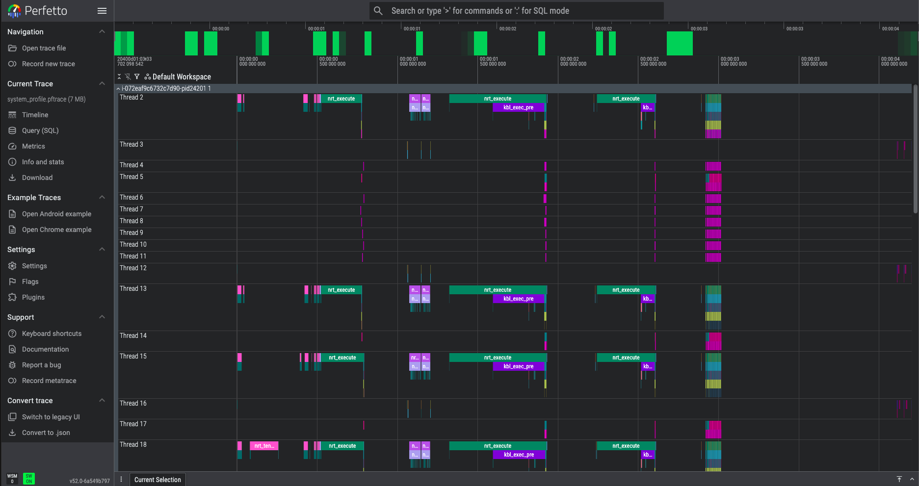
The system profile shows a high-level chronological view of the various Neuron Runtime API calls that took place during your example inference workload. If you hover the mouse cursor over the various pink/green bars you can see which specific API call occurred at each time point, such as nrt_tensor_read, nrt_tensor_write, nrt_execute, and nrt_load_collectives.

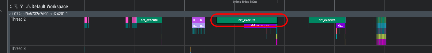
Look for the nrt_execute bar identified below and select it. This will open an information dialog providing details of the specific nrt_execute call:

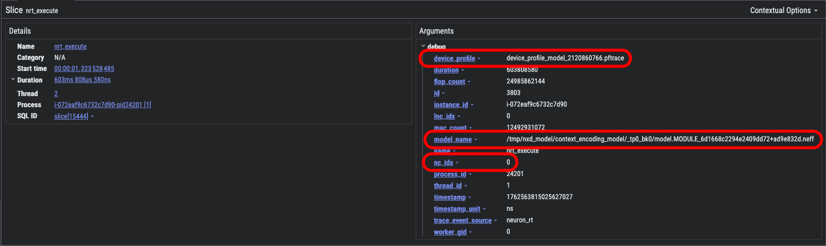
In the Arguments pane you will find useful information such as the following:

• device_profile - the unique name of the device profile associated with this event

• nc_idx - the index of the NeuronCore that is associated with this API call

• model_name - path to the compiled Neuron Executable File Format (NEFF) compute graph associated with this event

In the above screenshot, notice that the model_name field provides additional information about what is happening during this part of the model execution:

tmp/nxd_model/context_encoding_model/_tp0_bk0/model.MODULE_6d1668c2294e2409dd72+ad9e832d.neff

• context_encoding_model - indicates that this is handling context-encoding (prefill) during vLLM inference (other model names will alternatively include token_generation_model to indicate the token-generation / decode phase of inference).

• tp0 - indicates that this profile is associated with the rank0 of the tensor-parallel (TP) replica group

• bk0 - indicates that this profile is associated with the first sequence bucket as configured in Neuronx Distributed Inference (NxDI) NeuronConfig.

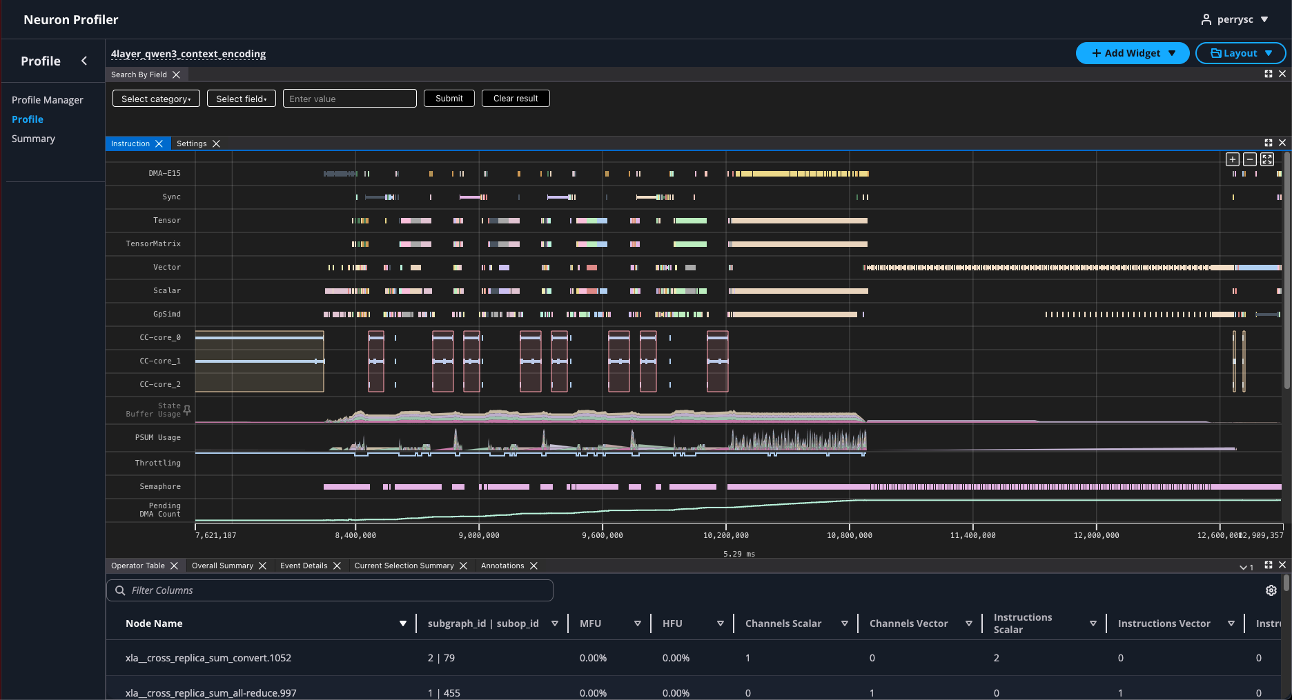
Step 4: Visualize device profiles in Neuron Explorer

In this step, you will view a device profile for your model in Neuron Explorer UI.

If you look inside the neuron_profiles directory that was created during Step 2, you will see many Neuron Executable File Format (NEFF) and their associated Neuron Trace File Format (NTFF) files. For each pair of NEFF/NTFF files, the NEFF represents the Neuron-compiled compute graph for a portion of your model, and the NTFF represents the device-level profile trace for that specific compute graph.

While you are free to view any of the device-level profiles using the Neuron Explorer UI, it is often more useful to start from the system-level profile and identify a specific device-level profile of interest. Let’s refer back to the nrt_execute region of the system-level profile that was covered in the previous section. Please find and left-click this region to bring up the information dialog at the bottom of Perfetto:

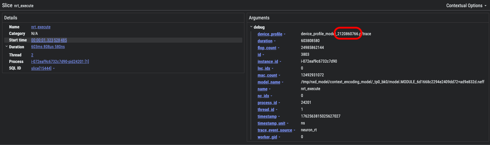
In the device_profile field, note that numerical ID that is included at the end of the device profile name, in this case 2120860766. This ID is what you will use to locate the NEFF/NTFF pair associated with this specific nrt_execute API call.

Use the following find command (substituting-in your device profile ID) to locate the NEFF/NTFF files associated with your identified ID:

find ./neuron_profiles -name \*2120860766\* | sort

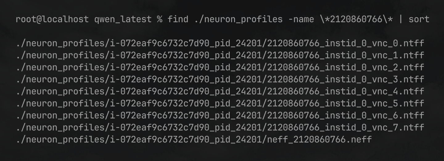
In the above output you can see that there is a single NEFF file neff_2120860766.neff, and multiple NTFF files 2120860766_instid_0_vnc_0.ntff … 2120860766_instid_0_vnc_7.ntff each representing the profile trace for one of the 8 NeuronCores that participated in this inference request.

These are the files you will open in the Neuron profiler UI to inspect the device-level execution.

Please copy the NEFF and one of the NTFF files to your local machine, as you will need to upload the files to the Neuron Explorer UI using your web browser.

To view the Neuron Profile Web UI, execute the view command to start the Neuron Explorer web UI:

$ neuron-profile view --data-path ./<workspace> --output-format parquet --ui-mode latest

<workspace> is a path that neuron-profile will use for storing and managing profiles.

The above command also prints a URL that you can click to open the web UI:

View a list of profiles at http://localhost:3001/

If neuron-profile view is run on a remote instance, you may need to use port forwarding to access the web UI. By default, neuron-profile creates a web server on port 3001 and the API server on port 3002. To enable connection to your browser on your local computer, you must to establish an SSH tunnel to both ports 3001 and 3002.

For example:

ssh -L 3001:localhost:3001 -L 3002:localhost:3002 <user>@<ip> -fN

If you created an EC2 instance with PEM credentials, include them in the SSH tunnel as seen below:

ssh -i ~/my-ec2.pem -L 3001:localhost:3001 -L 3002:localhost:3002 ubuntu@[PUBLIC_IP_ADDRESS] -fN

Once the SSH tunnel is setup, you can now open a browser and navigate to http://localhost:3001.

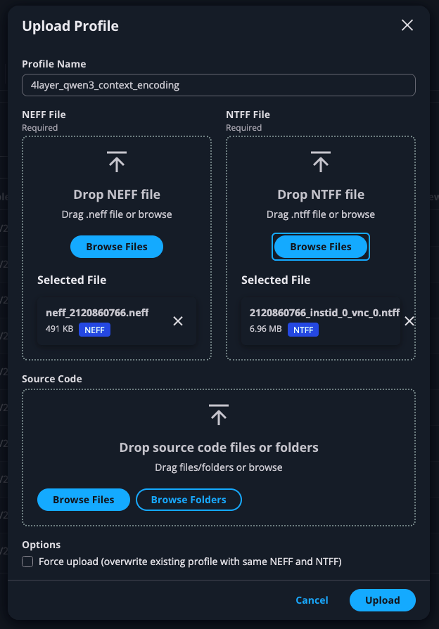
With the Neuron Explorer UI open, go to “Profile Manager”, and click “Upload Profile” at the top-right of the screen. Give your profile an appropriate name, and upload the NEFF and NTFF files that you previously identified:

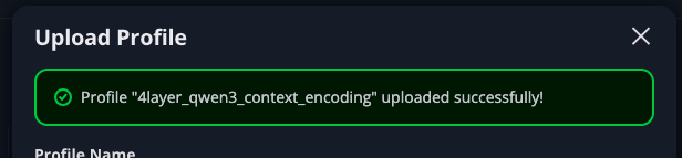
After a few seconds, you should receive a message indicating that NEFF/NTFF were uploaded successfully:

Within the Neuron Explorer UI, go tot he Profile Manager screen and look for your newly uploaded profile.

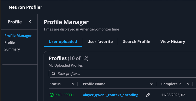
Depending on the size of your profile, it could take a few minutes before the Status field shows “PROCESSED”. Once processing is complete, click the profile name to open the profile:

Confirmation

Congratulations, you have now successfully generated both system-level and device-level profiles for a vLLM inference workload using Neuron Explorer and learned how to visualize them. This knowledge will enable you to effectively analyze the performance characteristics of your workload and identify potential optimization opportunities.

Clean up

After completing your profiling experiments, remember to terminate the instance you launched to avoid unnecessary costs.

Next steps

Now that you’ve completed this tutorial, try profiling your own model to analyze its workload. Identify performance gaps, apply optimizations, and profile again to measure the improvements. For a deeper dive into performance analysis, check out Neuron’s blog series on profiling.

This document is relevant for: Inf1, Inf2, Trn1, Trn2, Trn3