Disaggregated Inference [BETA]#

Overview#

Disaggregated Inference (DI), also known as disaggregated serving, disaggregated prefill, P/D disaggregation, is an LLM serving architecture that separates the prefill and decode phases of inference onto different hardware resources. To achieve this, the prefill worker needs to transfer the computed KV cache to the decode worker to resume decoding. Separating the compute intensive prefill phase from the memory bandwidth intensive decode phase can improve the LLM serving experience by

Removing prefill interruptions to decode from continuous batching to reduce inter token latency (ITL). These gains can be used to achieve higher throughput by running with a higher decode batch size while staying under Service Level Objectives (SLO).
Adapt to changing traffic patterns while still remaining under application SLOs.
Enable independent scaling of resources and parallelism strategies for prefill (compute bound) and decode (memory bound).

Note

Automatic Prefix Caching is not supported with DI.

High-Level Flow on Neuron#

Disaggregated Inference is mainly implemented through Neuron’s vLLM fork aws-neuron/upstreaming-to-vllm and the Neuron Runtime.

There are three main components to a DI workflow.

The router. Its job is to orchestrate requests to servers inside the prefill and decode clusters.
The prefill cluster. This represents all of the prefill servers ready to run a DI workload.
The decode cluster. This represents all of the decode servers ready to run a DI workload.

Below is an example lifespan of a single request through the DI flow.

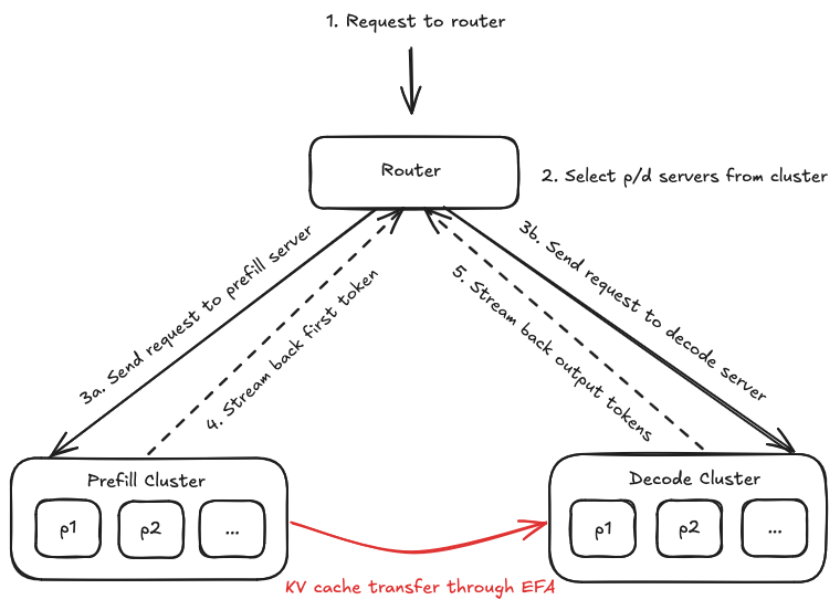
High Level Disaggregated Inference Architecture

1. A request is sent to the router (1), a component responsible for orchestrating (2) the requests to both the prefill and decode servers. It receives responses from the prefill and decode servers and streams the results back to the user.

2. The prefill server receives the request from the router (3a) and starts prefilling. After the prefill completes (4), it updates the status of the request for the decode server by sending information through another ZMQ server. Then, it listens for a “pull request” from the decode server to initiate the KV cache transfer. We use Neuron runtime APIs to transfer the KV cache through EFA from Neuron device to Neuron device. This is a zero copy transfer, meaning that we do not copy the KV cache from a Neuron device to CPU to transfer, but rather directly transfer KV cache from Neuron device to Neuron device. The transfer is also asynchronous. This means that the prefill server can immediately start prefilling the next request while the KV cache of the previous request is being transferred. This ensures that TTFT is not impacted for other requests while the KV cache for older request is being transferred to decode.

3. The decode server also receives a request from the router at the same time as the prefill server (3b). It waits until it receives a signal that its corresponding prefill is done from the prefill server by listening on the ZMQ server. Then, if there is a free spot in the decode batch, the scheduler will schedule the request and send a “pull request” to the prefill server. This initiates the asynchronous KV cache transfer (red arrow) through EFA by calling the Neuron Runtime API. The receive also needs to be asynchronous to ensure smooth ITL. While the receive is happening other decode requests will still run. As soon as the receive is finished the scheduler will add the request to the next decode batch (5).

Prefill Decode Interference When Colocating Prefill and Decode#

In traditional continuous batching, prefill requests are prioritized over decode requests. Prefills are run as batch size 1 because they are compute intensive whereas decodes can be run at a higher batch size because it is constrained on memory bandwidth not compute. To ensure the highest throughput, continuous batching schedulers prioritize new prefills if the decode batch is not at max capacity. As soon as a decode request finishes, another prefill is scheduled to fill the finished request’s place. However, all other ongoing decodes pause while the new prefill is running because that prefill uses the same compute resources. This effect is known as prefill stall or prefill contention.

Disaggregated Inference avoids prefill stall because the decode workflow is never interrupted by a prefill as it receives KV caches asynchronously while decoding. The overall ITL on DI is affected by the transfer time of the KV cache but this does not scale with batch size. For example, in a continuous batching workload of batch size 8 each request will on average be interrupted 7 times whereas in DI each request is only affected by a single transfer since it happens asynchronously.

Another advantage of DI is its ability to adapt to traffic patterns while maintaining a consistent ITL. For example, if prefill requests double in length the application can double the amount of available prefill servers in the prefill cluster to match the new traffic pattern. Continuous batching workloads would suffer because longer prefill requests increase tail ITL whereas DI workloads continue to deliver a low variance and a predictable customer experience.

Additionally, DI also allows users to tailor their parallelism strategies differently for prefill and decode. For example, a model with 32 attention heads may prefer to run two decode servers Data Parallel=2 (DP) each with Tensor Parallel=32 (TP) in order to reduce KV replication instead of TP=64. Such replication will get worse if using Group Query Attention (GQA).

DI does not necessarily improve throughput directly but it can help depending on the workload. Continuous batching is a technique optimized for throughput at the cost of ITL. An application may have an SLO to ensure that ITL is under a certain threshold. Because increasing the batch size increases the amount of prefill stall, and therefore increases ITL, many applications run on smaller than ideal batch sizes when using continuous batching. DI can allow an application to run at a higher batch size while still keeping ITL under the application defined SLO.

Trade-Offs#

Because DI runs prefill and decode separately, each part of the inference process needs to operate at an equal level of efficiency to maximize throughput and hardware resources. For example, if you can process 4 prefill requests per second and two decode requests per second the application will be stuck processing two requests per second. It is also important to note that the prefill and decode efficiency can vary based on the prompt length and the number of tokens for a response respectively. Continuous batching and chunked prefill do not have this issue as these techniques run prefill and decode on the same hardware.

One technique to remediate this is to run with a dynamic amount of prefill and decode servers. We call this dynamic xPyD. In the above example, we could run with 1 prefill and 2 decode servers so that our prefill and decode efficiency will be balanced.

Detailed System Overview#

Proxy Server Architecture#

The proxy server routes messages between clients and workers in our disaggregated inference system. It uses the Quart framework, Python’s asyncio libraries, and etcd to manage this communication.

Main Components#

Framework: Quart (for handling web requests)
Task Management: Python asyncio
Request Forwarding: Uses etcd to detect new prefill and decode workers (xPyD only)

How Requests Flow#

When a client sends a request, the proxy server starts two tasks at the same time:

prefill_task = asyncio.create_task(anext(prefill_response))
decode_task = asyncio.create_task(anext(decode_response))

await prefill_task
async for chunk in handle_prefill_response(prefill_response,
                                         streaming, endpoint,
                                         uid, request_time):
    yield chunk

await decode_task
async for chunk in handle_decode_response(decode_response,
                                        streaming, endpoint, uid,
                                        request_time):
    yield chunk

If running in static 1P1D mode, the workers are pre-chosen. If running in dynamic xPyD mode, the workers are chosen by round-robin and discovered through etcd.

This approach offers two benefits:

Faster responses because network delays don’t stack up
The decode server can get ready while prefill is working

How Tokens Work#

The proxy server handles tokens in specific ways to ensure accurate responses:

Prefill Settings#

Sets max_tokens=1 for prefill requests
Returns the first output token

Decode settings#

Runs as normal except it skips the first token from decode

Output Types#

The system can work in two ways decided by the client if streaming is enabled:

Streaming Mode
- Sends tokens to the client one at a time
- Uses both prefill and decode servers
- Shows results as they’re created
Batch Mode (stream=false)
- Sends all tokens at once when finished

Response Handling#

The proxy server:

Combines responses from both servers
Keeps tokens in the right order
Makes sure outputs match what clients expect from a regular system

Dynamic xPyD (Multiple Prefill, Multiple Decode)#

Dynamic xPyD lets you use multiple prefill and decode workers and dynamically add new workers to the cluster.

Note

The system can’t yet remove or handle unresponsive nodes automatically.

Worker Discovery and Connection Manager (neuron_connector.py)#

The system keeps track of workers using an etcd server. Here’s how it works:

class NeuronConnector:
    def _keep_alive_ectd(self):
        # Add worker to etcd
        etcd_client.put(
            f"/workers/{self.role}/{self.local_ip}/{self.api_server_port}",
            json.dumps({"connections": []}),
            lease
        )

This manager:

Signs up workers with etcd
Keeps a list of active connections
Creates new buffers when needed (dynamic xPyD)
Or statically creates buffers (static 1P1D)

Signal Plane (ZMQ Communication)#

Router (Prefill): Works with many decode connections
Dealer (Decode): Connects to prefill
Message Types:
- Welcome message when connecting
- Setting up key-value maps
- Managing transfers

Buffer Connection Management Details#

Buffer connection management is a critical component of the DI system that controls how servers communicate. The system supports two modes of operation: static 1P1D and dynamic xPyD. The connection management is done by neuron_connector.py and the actual buffer class is in neuron_buffer.py.

We use two types of buffers:

SendBuffer: For prefill workers
RecvBuffer: For decode workers

Static 1P1D Mode#

In static mode, the system creates a single buffer for each worker during initialization:

def initialize_buffer(self):
    if self.config.is_kv_producer:
        self.static_buffer = SendBuffer(
            self.kv_caches,
            self.zmq_context,
            self.neuron_recv_ip,
            self.config.kv_ip,
            self.config.kv_port
        )

This approach means:

All connection components are predefined
Communication paths are fixed
Buffers have predetermined communication partners

Dynamic xPyD Mode#

In dynamic mode, the system creates buffers on demand. Both SendBuffers and RecvBuffers can be created dynamically:

def maybe_setup_buffer(self, remote_ip, remote_port):
    if self.static_buffer:
        return self.static_buffer

    key = "" if self.config.is_kv_producer else (remote_ip, remote_port)

    if key in self.connection_dict:
        return self.connection_dict[key]

Key differences in dynamic mode:

One to many relationship between SendBuffers and RecvBuffers
Workers register themselves in etcd for service discovery
New connection determined by proxy server, the info is encoded in the request_id
Workers check their connection dictionary for existing buffers encoded in the request_id
If no buffer exists, they create a new one using the proxy server’s information
The new buffer establishes ZMQ communication with its partner

This dynamic approach allows the system to:

Add new connections as needed
Scale with changing workloads
Maintain efficient communication paths
Adapt to cluster changes

Transfer Engine and Communication#

Below is an image showing the KV cache transfer process on neuron:

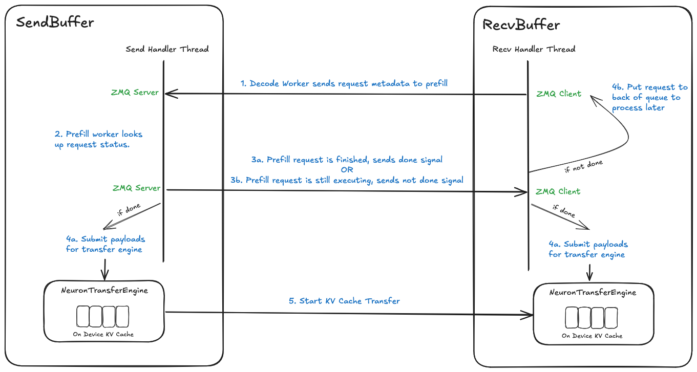
Transfer Engine (neuron_transfer_engine.py)#

The transfer engine moves KV cache efficiently between workers:

class NeuronTransferEngine:
    def transfer_neuron_tensors(self, tensors, offsets, lengths, peer_devices, ...):
        self.engine.queue_transfer_with_token(
            tensors, offsets, lengths, peer_devices, self.local_devices,
            self.comm_ids, completion_count, completion_token, use_queue,
            completion_time_out)

The engine:

Sets up KV communication between devices
Calls Neuron Runtime APIs to move KV caches
Tracks when transfers finish

Zero-Copy Transfer System#

Runs in its own thread
Listens for requests from decode servers
Handles three types of requests:
- Handshakes to confirm connection establishment
- Setting up KV cache maps
- Decode server requests for KV cache transfer (lookup_all)

Here’s how it works:

def send_handler(self):
    while True:
        identity, request = self.router.recv_json()

        if request["type"] == "handshake":
            self.router.send_json(identity, {
                "status": "ok",
                "timestamp": time.time()
            })
            continue

        if request["type"] == "kv_map_init":
            # Set up transfer details
            continue

        if request["type"] == "lookup_all":
            self._process_lookup_all(identity, request)
            continue

Keeps a list of waiting transfers
For each task:
- Sends request to prefill server
- Waits for answer
- If successful:
  - Saves the output token from signal plane
  - Starts moving the KV cache through Transfer Engine
- If it fails:
  - Tries again later

On the Prefill Side:

# ensure that the request is finished prefill
if request_id not in self.lookup_dict:
    self.router.send_json(identity, {"success": False})
    return

# After getting decode server request and prefill is finished
kv_caches, offsets, lengths, peer_devices = \
    self.generate_transfer_sequences(entry, remote_id=identity_str)

# Start transfer
self.get_transfer_engine(remote_id=identity_str).transfer_neuron_tensors(
    kv_caches, offsets, lengths, peer_devices,
    completion_token=entry.completion_token)

On the Decode Side:

# receive prefill worker's output token
entry.output_token = torch.tensor(
    response["output_token"]).unsqueeze(0)

kv_caches, offsets, lengths, peer_devices = \
     self.generate_transfer_sequences(entry)

# do not wait for request completion for recv buffer
self.get_transfer_engine().transfer_neuron_tensors(
    kv_caches, offsets,lengths, peer_devices,
    completion_token=entry.completion_token)

The completion_token provides the status of the transfer.

Note

These are separate threads from the main inference process and do not block ongoing inference.

Request Scheduling Rules#

Here are new scheduling rules for Disaggregated Inference:

Prefill Worker Rules#

Requests can be: Waiting, Transferring, or Running
Only one request can run at a time
Total of transferring + running must not exceed batch size
Can start new requests when:
- Nothing is running
- Number of transfers is less than batch size

Decode Worker Rules#

Uses same request states as prefill
Running + transferring must not exceed batch size
Running must not exceed batch size
Must finish key-value cache transfer before running
Can start new transfers when there’s space

Scheduler Jobs#

Adds transfer requests to a list
Checks status without blocking
Uses status to make decisions
Doesn’t handle transfers directly

These rules help:

Keep key-value caches safe
Use resources well
Process batches efficiently
Keep scheduling separate from transfers

Example Usage#

Refer to the offline inference DI example for a quick example to get started.

Refer to the Disaggregated Inference Tutorial for a detailed usage guide.

Disaggregated Inference [BETA]

Contents

Disaggregated Inference [BETA]#

Overview#

High-Level Flow on Neuron#

Prefill Decode Interference When Colocating Prefill and Decode#

Trade-Offs#

Detailed System Overview#

Proxy Server Architecture#

Main Components#

How Requests Flow#

How Tokens Work#

Prefill Settings#

Decode settings#

Output Types#

Response Handling#

Dynamic xPyD (Multiple Prefill, Multiple Decode)#

Worker Discovery and Connection Manager (neuron_connector.py)#

Signal Plane (ZMQ Communication)#

Buffer Connection Management Details#

Static 1P1D Mode#

Dynamic xPyD Mode#

Transfer Engine and Communication#

Transfer Engine (neuron_transfer_engine.py)#

Zero-Copy Transfer System#

Request Scheduling Rules#

Prefill Worker Rules#

Decode Worker Rules#

Scheduler Jobs#

Example Usage#