This document is relevant for: Inf2, Trn1, Trn2
Deep dive: Explore Mixture of Experts (MoE) inference support for Neuron#
Why read this guide? This guide is intended for ML engineers looking to implement custom MoE models or implement advanced performance optimizations on Neuron. It explains how each MoE component maps to Neuron hardware and how to combine router, expert, and parallelism settings to extract maximium performance during the prefill and decode phases of MoE model inference.
How to use this guide: If you are looking to deploy existing MoE models with vLLM, refer to the vLLM user guide instead. Skip to the optimization sections if you already know NxD basics.
This topic explores Mixture of Experts (MoE) inference in depth. It discusses the technical details from an AWS Neuron expert perspective. You need experience with model sharding concepts like Tensor Parallelism and performance tuning on Neuron using Neuron Kernel Interface (NKI) to fully understand this content.
Prerequisites#
Before you start, you must be familiar with the following:
NxD Inference library overview: How to build and deploy models using NxD Inference. See NxD Inference.
Neuron Kernel Interface (NKI): Performance optimization techniques using NKI for custom kernel development. See Neuron Kernel Interface (NKI).
Model parallelism techniques: Tensor parallelism and other distributed inference strategies. See Parallelism Techniques for LLM Inference.
Overview#
Mixture of Experts (MoE) is a neural network architecture that scales to massive parameter counts while maintaining computational efficiency. An MoE layer replaces a traditional dense feedforward network with multiple specialized “expert” networks. Only a subset of experts are activated per token. Each input token is processed by only the top-k most relevant experts (typically k=1-8), as determined by a learned router. This selective activation allows models to have billions of parameters while computing only a fraction of them. This breaks the linear relationship between model size and computational cost. Due to its computational benefits, the MoE architecture has gained significant adoption across the industry. Recent models like GPT-OSS, Llama4, DeepSeek-V3, and Qwen3-MoE all use MoE.
Implementing MoE models to extract peak performance on Neuron hardware requires careful design. This is due to the dynamic nature of expert selection, which creates variable computational graphs. These must be handled within Neuron’s static compilation model. Expert routing decisions vary per iteration. This causes different number of tokens to be assigned to each expert. This requires algorithms like the blockwise matrix multiplication approach to maintain static tensor shapes while minimizing padding overhead. Additionally, MoE models require careful consideration of tensor parallelism (TP), expert parallelism (EP), and sequence parallelism (SP) strategies. The optimal approach depends on expert size, sparsity patterns, and whether the workload is compute-bound (prefill) or memory-bound (decode). These topics form the focus of this deep dive.
Anatomy of an MoE layer and MoE API in NxDI#
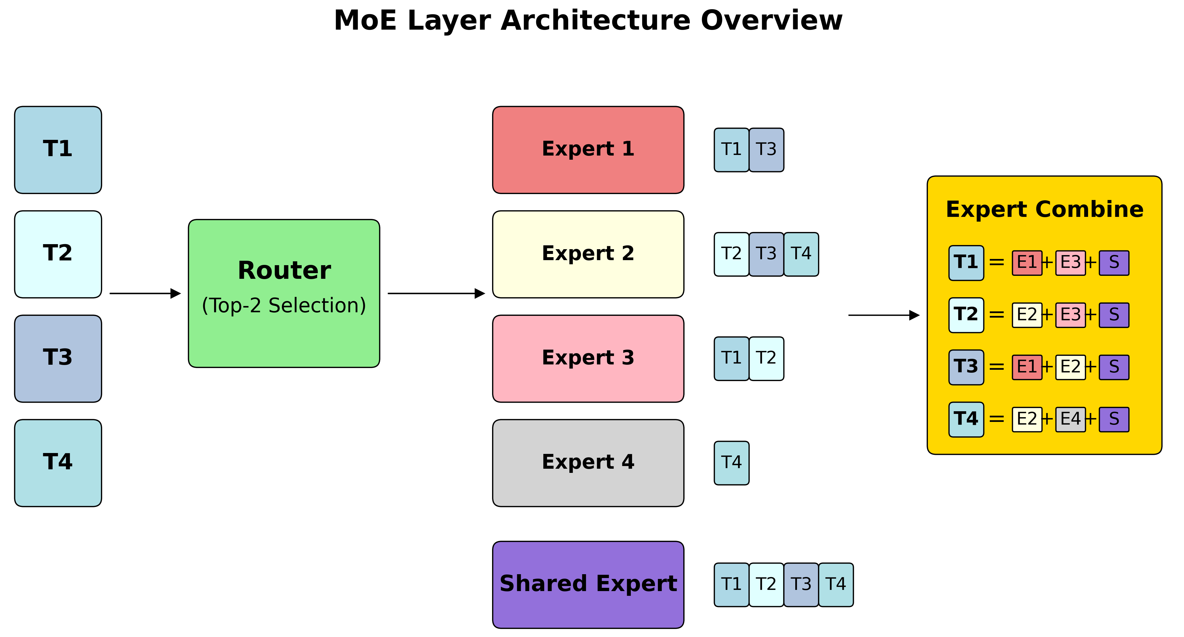
An MoE layer consists of three main components: a router that determines expert selection, expert MLPs that perform the actual computation, and optional shared experts that process all tokens. The NxD Inference library provides a comprehensive set of APIs for building MoE layers that mirrors this conceptual structure.
MoE Layer Structure#
The MoE class in NeuronxDistributed serves as the main orchestrator. It combines the
three core components into a unified layer. The data flow implements a clear pattern:
input tokens first pass through the router to determine expert assignments, then through
the selected expert MLPs for computation, and finally through optional shared experts
before output combination. This modular design allows you to flexibly configure and
build different MoE model architectures. You also benefit from optimizations in the
Neuron SDK to optimize MoE model performance.
Expert combine is an operation where outputs from multiple experts are weighted and combined to produce the final token representation. For each token processed by top-k experts, the router produces affinity scores that determine how much each expert’s output contributes to the final result. Mathematically, for a token processed by experts \(E_1, E_2, ..., E_k\) with corresponding affinities \(a_1, a_2, ..., a_k\), the final output is computed as:
where:
\(E_i(\text{token})\) is the output of expert \(i\) for the given token
\(a_i\) is the affinity score for expert \(i\)
\(k\) is the number of selected experts (top_k)
This weighted combination ensures that experts with higher routing confidence contribute
more significantly to the final output. The affinity normalization (controlled by
normalize_top_k_affinities) ensures that \(\sum_{i=1}^{k} a_i = 1.0\) across the selected
experts for each token. The NxD framework handles this expert combination logic internally,
along with routing and static compilation optimizations.
Below is an example of how to instantiate the MoE API:
from neuronx_distributed.modules.moe import MoE, routing
from neuronx_distributed.modules.moe.expert_mlps_v2 import ExpertMLPsV2
from neuronx_distributed.modules.moe.moe_configs import (
    RoutedExpertsMLPOpsConfig,
    BlockwiseMatmulConfig
)
from neuronx_distributed.modules.moe.shared_experts import SharedExperts

# Example: GPT-OSS MoE layer configuration
num_experts = 128
top_k = 8
hidden_size = 7168
intermediate_size = 2048

# Initialize router for expert selection
router = routing.RouterTopK(
    num_experts=num_experts,
    top_k=top_k,
    hidden_size=hidden_size,
)

# Configure expert MLPs using ExpertMLPsV2 class
routed_experts_config = RoutedExpertsMLPOpsConfig(
    num_experts=num_experts,
    top_k=top_k,
    hidden_size=hidden_size,
    intermediate_size=intermediate_size,
    hidden_act="silu",
    glu_mlp=True,
    capacity_factor=None,  # Full capacity, no token dropping
    normalize_top_k_affinities=True,
)

# These configs relate to the blockwise matrix multiply (BWMM) algorithm,
# which enables static compilation by organizing tokens into fixed-size blocks
# assigned to experts. BWMM tuning parameters are covered in detail later.
blockwise_config = BlockwiseMatmulConfig.from_kwargs(
    block_size=512,
    logical_nc_config=2,  # Use LNC2 for Trn2
)

expert_mlps = ExpertMLPsV2(
    routed_experts_mlp_config=routed_experts_config,
    blockwise_matmul_config=blockwise_config,
    sequence_parallel_enabled=True,
)

# Create complete MoE layer
moe_layer = MoE(
    router=router,
    expert_mlps=expert_mlps,
    sequence_parallel_enabled=True,
)
Router#
The router component determines which experts compute each token through routing
decisions learned during model training. NxD Inference supports multiple routing
strategies, each optimized for different model architectures. The RouterBase
class provides interfaces for inputs and outputs that the MoE module expects. Specialized implementations offer distinct
routing behaviors.
The RouterTopK implementation available for use out of the box in NxD inference provides standard top-k expert selection, making it
suitable for most MoE models including GPT-OSS, Llama4, and Qwen-3 Moe. It supports
both softmax and sigmoid activation functions for computing token to expert affinities:
# Standard top-k routing (used in GPT-OSS, DBRX)
router = routing.RouterTopK(
    num_experts=128,
    top_k=8,
    hidden_size=7168,
    act_fn="softmax",  # or "sigmoid"
    sequence_parallel_enabled=True,
)
The GroupLimitedRouter is another built-in routing API that implements the no-auxiliary-loss method from DeepSeek-V3,
which groups experts and selects top groups before performing top-k selection within
those groups:
# Setting up Group-limited routing (DeepSeek-V3 style)
router = routing.GroupLimitedRouter(
    num_experts=256,
    top_k=8,
    hidden_size=7168,
    n_group=8,  # Number of expert groups
    topk_group=2,  # Top groups to select
)
Routed Experts#
The ExpertMLPsV2 class handles the core routed expert computation. It computes tokens through
their assigned experts. This class contains implementations of the experts matrix
multiplication that are optimized depending on whether the workload is compute-bound
or memory-bound. It automatically selects the appropriate strategy based on sequence
length, batch size and other architectural parameters.
The V2 API provides a configuration-based approach with RoutedExpertsMLPOpsConfig
for expert-specific settings to implement different MoE architectures
and BlockwiseMatmulConfig for optimization parameters.
This separation provides cleaner configuration management and better extensibility:
# GPT-OSS Expert MLPs configuration
routed_experts_config = RoutedExpertsMLPOpsConfig(
    num_experts=128,
    top_k=8,
    hidden_size=7168,
    intermediate_size=2048,
    hidden_act="swiglu",
    glu_mlp=True,
    capacity_factor=None,  # Full capacity, no token dropping
    normalize_top_k_affinities=True,
)

# Configuration parameters for the BWMM algorithm, which are explained later.
blockwise_config = BlockwiseMatmulConfig.from_kwargs(
    block_size=512,
    logical_nc_config=2,  # Use LNC2 for Trn2
    skip_dma_token=True,  # Skip loading padded tokens
    skip_dma_weight=True,  # Skip duplicate weight loads
)

expert_mlps = ExpertMLPsV2(
    routed_experts_mlp_config=routed_experts_config,
    blockwise_matmul_config=blockwise_config,
    sequence_parallel_enabled=True,
)
NxD Inference supports both dropping and dropless MoE strategies. Each has different
trade-offs between computational efficiency and model accuracy. The choice between these
strategies is controlled by the capacity_factor parameter in the expert configuration.
Dropless MoE (capacity_factor=None) processes all tokens through their assigned
experts without dropping any tokens. This approach maintains full model accuracy but
requires dynamic handling of variable expert loads. Models using dropless strategies
include GPT-OSS, Llama4, and DBRX. The blockwise matrix multiplication
algorithm enables efficient dropless computation by organizing tokens into fixed-size
blocks while minimizing padding overhead:
# Dropless MoE configuration (recommended for inference)
routed_experts_config = RoutedExpertsMLPOpsConfig(
    num_experts=128,
    top_k=8,
    hidden_size=7168,
    intermediate_size=2048,
    hidden_act="swiglu",
    glu_mlp=True,
    capacity_factor=None,  # Dropless - no tokens dropped
    normalize_top_k_affinities=True,
)
Dropping MoE (capacity_factor > 0) sets a fixed capacity for each expert and
drops tokens that exceed this capacity. This approach provides more predictable
computational costs but may impact model accuracy due to dropped tokens. Models using
dropping strategies include DeepSeek-V3:
# Dropping MoE configuration with 25% extra capacity
routed_experts_config = RoutedExpertsMLPOpsConfig(
    num_experts=128,
    top_k=8,
    hidden_size=2880,
    intermediate_size=2880,
    hidden_act="swiglu",
    glu_mlp=True,
    capacity_factor=1.25,  # 25% extra capacity beyond perfect balance
    normalize_top_k_affinities=True,
)
Parallelism Strategies for Routed Experts
MoE models on Neuron hardware benefit from two primary parallelism strategies that can be used independently or in combination to optimize performance and memory usage:
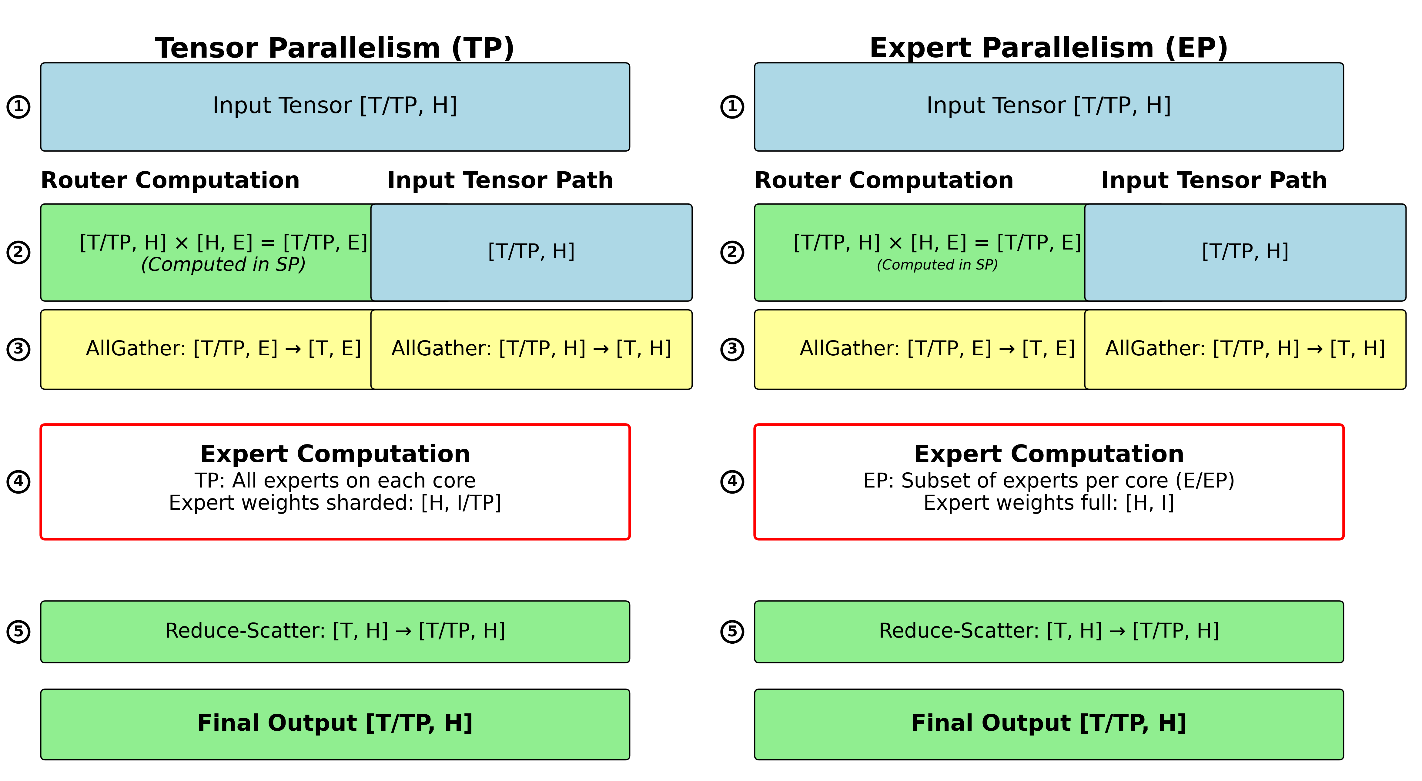
Tensor Parallelism (TP) distributes each expert’s computation across multiple NeuronCores by sharding the expert weights along the intermediate dimension. This approach reduces memory usage per core and enables larger models to fit in available memory. With TP, each expert’s gate, up, and down projection matrices are split across TP ranks, requiring collective communication to combine results.
Expert Parallelism (EP) distributes different experts across different NeuronCores, allowing each core to specialize in computing a subset of the total experts.
As we discuss later in this deep dive, the choice between TP and EP (or their combination) depends on model architecture and the specific TRN hardware under consideration.
To configure TP and EP, configure the degrees while initializing the model parallel state in NxD. The MoE components automatically create and use the appropriate PyTorch process groups based on the parallelism configuration. These configurations set up routed expert behavior and parallelism strategy, while NxD internally manages mapping to the optimized kernels, and process group mapping for TP/EP. We show a few code examples below.
from neuronx_distributed.parallel_layers import parallel_state

# Configure Tensor Parallelism only (TP=8)
parallel_state.initialize_model_parallel(
    tensor_model_parallel_size=8,
    expert_model_parallel_size=1,  # No expert parallelism
)

# Configure Expert Parallelism only (EP=16)
parallel_state.initialize_model_parallel(
    tensor_model_parallel_size=1,  # No tensor parallelism
    expert_model_parallel_size=16,
)

# Configure combined TP and EP (TP=4, EP=16)
parallel_state.initialize_model_parallel(
    tensor_model_parallel_size=4,
    expert_model_parallel_size=16,
)
MoE prefill optimization#
This section explores the core design principles and optimization techniques that enable efficient MoE execution during prefill. It focuses on three key areas: router execution strategies, blockwise matrix multiplication algorithms for efficient routed expert computation, and optimization strategies for shared experts.
Router execution in sequence parallel mode#
Router networks are significantly smaller compared to expert MLPs. They have weight matrices of size \([\mathrm{hidden\_size}, \mathrm{num\_experts}]\). For most MoE architectures, this represents a relatively modest memory footprint that allows RouterTopK to run with replicated weights across sequence parallel ranks. NxD also delays logit gathering until after expert selection to reduce communication volume. Consider a concrete example:
Example: GPT-OSS 120B configuration
- Hidden size: 2880
- Number of experts: 128
- Router weight size: 2880 × 128 × 2 bytes = ~0.07MB per MoE layer
- Router across all layers: 0.07MB × 36 layers = ~2.4MB
- Replicating the router occupies ~0.01% of HBM capacity on a TRN2 instance
The small size of router weights makes weight replication across cores acceptable. This enables sequence parallel execution where each core processes a subset of the sequence but maintains a complete copy of the router weights. This approach improves the arithmetic intensity of router layer operations without imposing significant memory overhead.
Communication optimization in sequence parallel mode
The NxD implementation performs an additional optimization to reduce communication overhead. A naive implementation of router in sequence parallel (SP) would involve gathering the router logits computed in sequence parallel. This induces a communication volume of \([\mathrm{batch\_size}, \mathrm{seq\_len}, \mathrm{num\_experts}]\). The gathering of logits is needed to proceed to the next step of computing experts. The computation operates in TP or EP mode rather than SP. For long sequences and models with a large number of experts, this step can become a performance bottleneck.
To optimize this, we delay gathering logits until after expert selection is completed. Following this step, the size of router logits to be gathered becomes \([\mathrm{batch\_size}, \mathrm{seq\_len}, \mathrm{top\_k}]\). This is significantly smaller and reduces communication overhead by a factor of \(\frac{\mathrm{num\_experts}}{\mathrm{top\_k}}\).
For example, with 128 experts and top_k=8, this optimization reduces communication volume by 16×.
Takeaway: During prefill, we recommend configuring the router in sequence parallel mode.
Enabling router in sequence parallel mode
The router implementation in NxD automatically handles sequence parallel execution through
the sequence_parallel_enabled parameter.
# Router configuration for sequence parallel execution
router = routing.RouterTopK(
    num_experts=128,
    top_k=8,
    hidden_size=2880,
    sequence_parallel_enabled=True,  # Enable SP execution
    act_fn="softmax"
)
Blockwise Matrix Multiplication (BWMM): Routed Expert optimization#
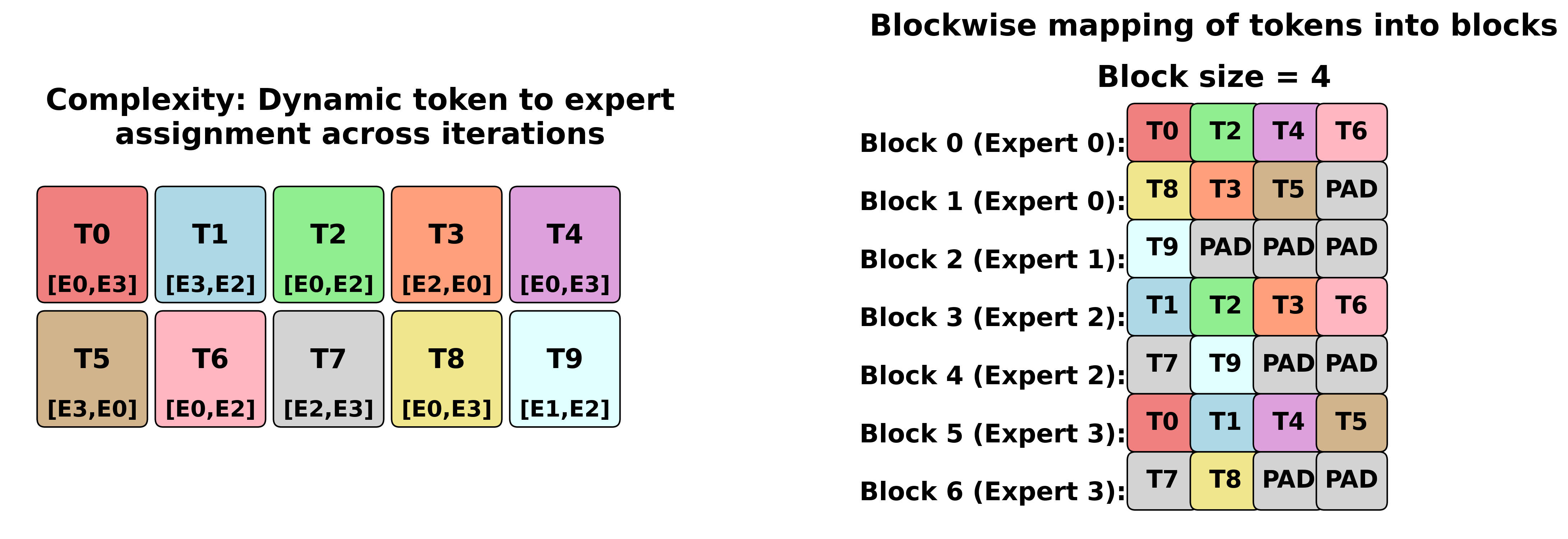
A naive implementation of routed expert computation inherently creates dynamic computational graphs. This is because token-to-expert distributions vary across iterations.
Consider a simple example that illustrates the core problem:
# Naive MoE implementation picked from HuggingFace
# (problematic for static compilation)
def moe_forward(tokens, experts, router):
    expert_assignments = router(tokens)  # Dynamic routing decisions
    outputs = []

    for expert_id in range(num_experts):
        # Variable number of tokens per expert each iteration
        expert_tokens = tokens[expert_assignments == expert_id]
        if len(expert_tokens) > 0:
            # experts[expert_id] represents the expert network/function
            expert_output = experts[expert_id](expert_tokens)
            outputs.append(expert_output)

    return combine_outputs(outputs, expert_assignments)
Blockwise matrix multiplication solution#
The blockwise matrix multiplication (BWMM) approach solves this challenge by transforming the dynamic problem into a static one. It maps tokens into fixed-size computational blocks:
Core design principles:
The algorithm maps tokens into blocks with a fixed number of tokens (equal to block_size). It maintains the following constraints:
Single expert per block: Each block contains tokens assigned to only one expert
Multiple blocks per expert: Experts can be assigned multiple blocks when needed
Padded blocks allowed: Some blocks may contain only padding tokens depending on the token-to-expert distribution during inference
For dropless inference, provisioning \(N = \lceil\frac{\mathrm{tokens} \times \mathrm{top\_k}}{\mathrm{block\_size}}\rceil + (\mathrm{num\_experts} - 1)\) blocks is sufficient to map all tokens without dropping while satisfying these constraints.
Concrete example:
Input: 6 tokens [T0, T1, T2, T3, T4, T5]
Expert assignment: [E0, E1, E0, E2, E1, E0]
Block size: 4

Block organization:
Block 0 → Expert E0: [T0, T2, T5, -1]  # 3 real tokens + 1 padding
Block 1 → Expert E1: [T1, T4, -1, -1]  # 2 real tokens + 2 padding
Block 2 → Expert E2: [T3, -1, -1, -1]  # 1 real token + 3 padding
Padding overhead analysis
Understanding padding overhead is crucial for optimizing MoE performance. It directly impacts compute utilization and memory efficiency. The BWMM algorithm introduces padding in two scenarios: within blocks (when experts receive fewer tokens than block_size) and across blocks (when we provision more blocks than the minimum required).
Mathematical framework:
The total padding overhead can be quantified as:
Where:
\(N\) = number of blocks provisioned
\(T\) = total input tokens
\(\mathrm{block\_size}\) = tokens per block
\(\mathrm{top\_k}\) = experts per token
Concrete example - Padding impact:
Scenario: 1000 tokens, 8 experts, top_k=2, block_size=256

Required computation: 1000 × 2 = 2000 token-expert pairs

Blocks statically provisioned to handle worst case:
N = ⌈(1000 × 2) / 256⌉ + (8 - 1) = ⌈7.8⌉ + 7 = 15

Best case (perfect load balancing):
- Each expert gets: 2000 ÷ 8 = 250 tokens
- Blocks needed: 8 experts × 1 block = 8 blocks
- Total compute slots (required): 8 × 256 = 2048
- Total compute slots (actual): 15 × 256 = 3840
- Padding overhead (to handle worst case): (3840 - 2048) ÷ 2048 = 87.5%
- Algorithmic padding overhead: (2048 - 2000) / 2000 = 2.4%

Worst case (load imbalance):
- One expert gets 1750 tokens, others get ~36 tokens each
- Blocks needed: 7 blocks for hot expert + 7 blocks for others = 14 blocks
- Total compute slots (required): 14 × 256 = 3584
- Total compute slots (actual): 15 × 256 = 3840
- Padding overhead (to handle worst case): (3840 - 3584) ÷ 3584 = 7.14%
- Algorithmic padding overhead: (3584 - 2000) / 2000 = 79.2%
Block size selection guidance
Trade-offs:
Smaller block_size (e.g., 128):
✓ Reduces within-block padding, improving performance when token-to-expert distribution is imbalanced
✗ Lower arithmetic intensity per block

Larger block_size (e.g., 1024):
✓ Higher arithmetic intensity per block
✗ Higher within-block padding for sparse experts
Optimization principle:
Choose the block size just large enough so that the workload becomes compute-bound rather than memory-bound.
The arithmetic intensity factor (AIF) provides a quantitative framework for block size selection:
Target configuration: \(\text{AIF} \geq \frac{\text{Peak compute throughput}}{\text{Memory bandwidth}}\)
For TRN2 instances, this ratio is approximately 400-500 FLOPs/byte, providing guidance for optimal block size selection.
Advanced optimizations in the BWMM algorithm#
The implementation of the BWMM kernel that is available in the Neuron SDK provides several sophisticated optimizations. These significantly improve MoE performance by reducing memory bandwidth requirements and eliminating unnecessary computation.
DMA skipping optimizations
DMA (Direct Memory Access) skipping addresses the padding overhead inherent in the blockwise approach. It selectively avoids DMA transfers for padded elements.
Token skipping:
Token skipping eliminates memory transfers for padded token positions (marked as -1 in
the token position mapping):
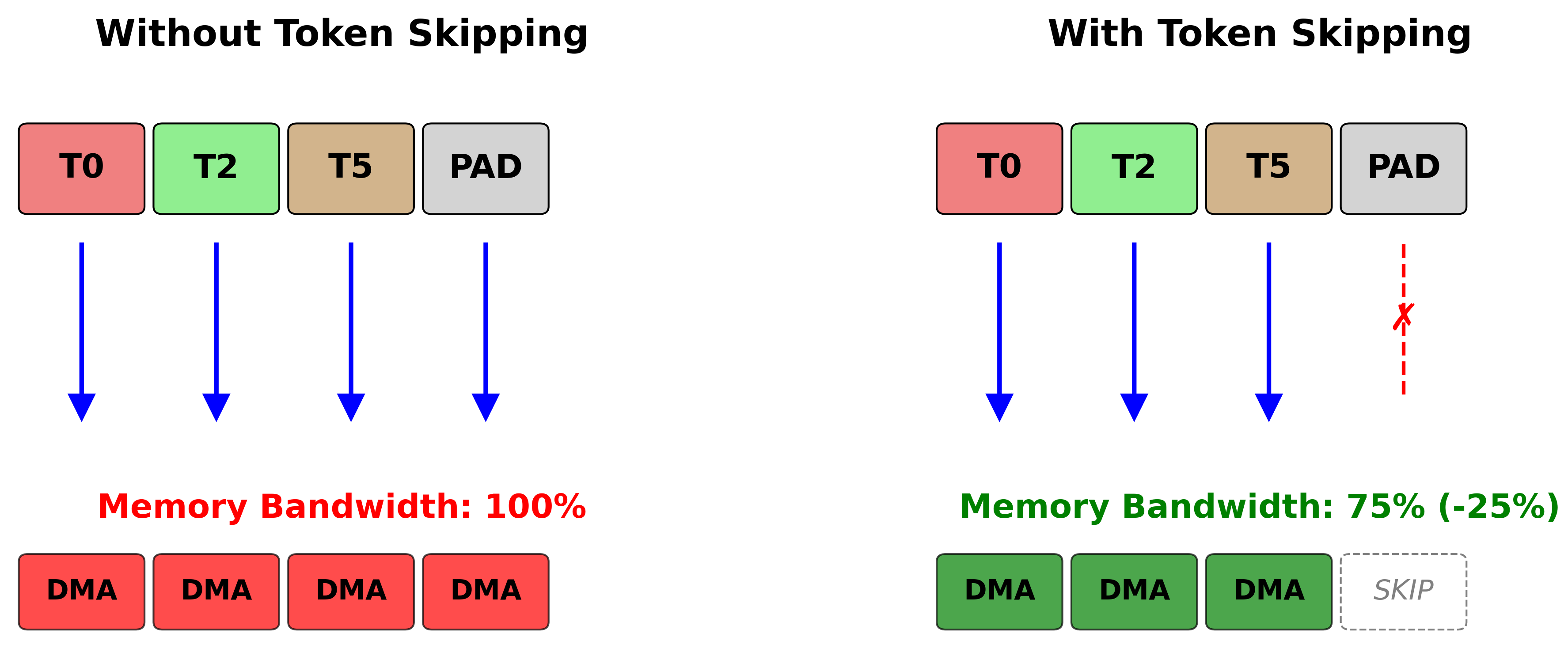
Without token skipping:
Block: [T0, T2, T5, -1]
DMA operations: 4 token loads (including padding)

With token skipping:
Block: [T0, T2, T5, -1]
DMA operations: 3 token loads (padding skipped)
Performance improvement: ~25% reduction in memory bandwidth
Weight skipping:
Weight skipping avoids redundant expert weight loads when consecutive blocks use the same expert:
Block sequence: [E0, E0, E1, E2, E2]

Without weight skipping:
- Load E0 weights for Block 0
- Load E0 weights for Block 1 (redundant)
- Load E1 weights for Block 2
- Load E2 weights for Block 3
- Load E2 weights for Block 4 (redundant)

With weight skipping:
- Load E0 weights for Block 0
- Reuse E0 weights for Block 1
- Load E1 weights for Block 2
- Load E2 weights for Block 3
- Reuse E2 weights for Block 4
Configuration in NxD Inference:
Recommendation is to have both these features as default on.
# Enable DMA skipping optimizations
blockwise_config = BlockwiseMatmulConfig.from_kwargs(
    block_size=512,
    logical_nc_config=2,
    skip_dma_token=True,    # Enable token skipping
    skip_dma_weight=True,   # Enable weight skipping
)
Dynamic control flow - block compute skipping
Dynamic control flow optimization eliminates computation entirely for blocks that contain only padding tokens. This is done inside the kernel by leveraging support for executing while loops on chip with dynamic number of iterations in the Neuron SDK.
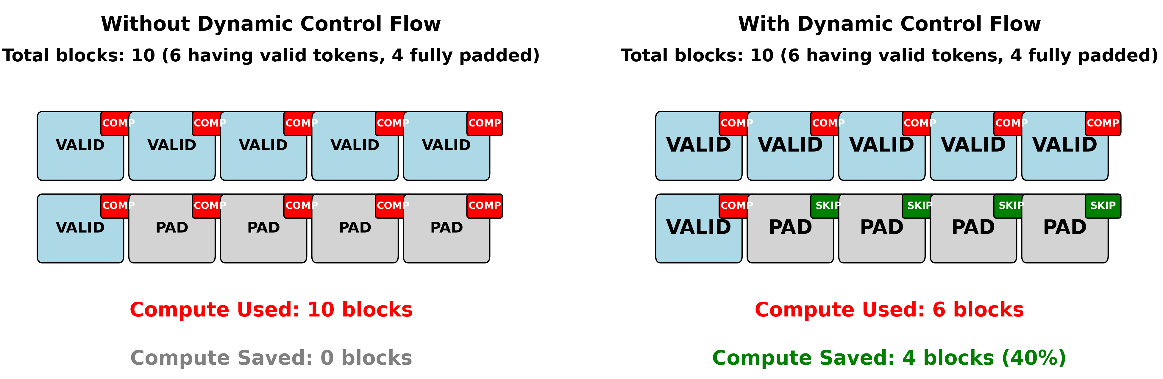
Conceptual example:
Total blocks: 10
Token distribution: 6 blocks with real tokens, 4 blocks fully padded

Block to expert allocation: [1, 1, 1, 1, 1, 1, 0, 0, 0, 0]
                           ^-- real blocks --^  ^-- skip --^

Regular execution: Compute all 10 blocks
With dynamic control flow: Compute only 6 blocks, skip 4 entirely
Performance improvement roofline: ~40% reduction in compute FLOPs, especially when token to expert distribution is not imbalanced.
NxD Inference configuration:
# Enable dynamic control flow optimization
blockwise_config = BlockwiseMatmulConfig.from_kwargs(
    block_size=512,
    logical_nc_config=2,
    # Choose based on LNC2 sharding:
    use_shard_on_block_dynamic_while=True,
    # OR
    use_shard_on_intermediate_dynamic_while=True, # Based on technique used for LNC2 sharding
)
LNC2 sharding strategies
TRN2 and TRN3 provide two physical cores per logical NeuronCore. NxD inference via the Neuron Kernel Library (NKI-Lib) supports three distinct sharding strategies, each optimized for different scenarios. The choice of LNC sharding algorithm can be configured through BlockwiseMatmulConfig parameters:
Hidden dimension sharding (shard on H):
Default sharding strategy in BlockwiseMatmulConfig.
Computation per block: [block_size, H] @ [H, I] @ [I, H]
Sharding strategy: Split H dimension across cores

Core 0: [block_size, H/2] @ [H/2, I] @ [I, H/2]
Core 1: [block_size, H/2] @ [H/2, I] @ [I, H/2]

Requires: Cross-core reduction after first matmul
Best for: High tensor parallelism scenarios
Intermediate dimension sharding (shard on I):
Configured with use_shard_on_intermediate_dynamic_while=True in BlockwiseMatmulConfig.
Computation per block: [block_size, H] @ [H, I] @ [I, H]
Sharding strategy: Split I dimension across cores

Core 0: [block_size, H] @ [H, I/2] @ [I/2, H]
Core 1: [block_size, H] @ [H, I/2] @ [I/2, H]

Requires: Cross-core reduction after second matmul
Best for: Low expert parallelism scenarios, large intermediate dimensions
Block parallel execution:
Configured with use_shard_on_block_dynamic_while=True in BlockwiseMatmulConfig.
Total blocks: N
Sharding strategy: Distribute blocks across cores

Core 0: Processes blocks [0, 2, 4, ...] (even indices)
Core 1: Processes blocks [1, 3, 5, ...] (odd indices)

Requires: Enough HBM capacity to store intermediate outputs across cores and a cross-core reduction at the end.
Best for: When workload can afford the HBM capacity to store intermediate outputs from both cores and when there is more than one expert per logical core.
Configuring TP and EP#
The choice between Tensor Parallelism (TP) and Expert Parallelism (EP) depends on several model characteristics and hardware constraints. This section provides practical guidance for selecting the optimal parallelism strategy.
Decision framework
When to prefer Tensor Parallelism:
Small number of experts (≤32): TP provides good load balancing without expert distribution concerns
Large intermediate dimensions: Optimal configuration is when sharded intermediate dimensions are >= 128 for good tensor engine utilization
When to prefer Expert Parallelism:
Large number of experts (≥64): Better expert distribution and load balancing
Small intermediate dimensions: Avoids under-utilization from excessive TP sharding
Hybrid TP+EP approach:
Best of both worlds: Combine moderate TP (2-8) with EP to achieve good compute efficiency.
Load balancing problem with very large EP: Expert parallelism can suffer from load imbalance.
Some EP groups receive significantly more work than others. In the worst case, one EP group may receive 3-4x the average number of tokens. This creates straggler effects that limit overall performance. This skew becomes more pronounced with larger EP degrees and imbalanced routing patterns. The overall MoE layer performance is determined by the slowest EP group. This makes load balancing critical for EP effectiveness.
Configuration examples
# Small model, balanced routing - prefer TP
parallel_state.initialize_model_parallel(
    tensor_model_parallel_size=8,
    expert_model_parallel_size=1,
)

# Large model, many experts - prefer EP
parallel_state.initialize_model_parallel(
    tensor_model_parallel_size=1,
    expert_model_parallel_size=16,
)

# Very large model - hybrid approach
parallel_state.initialize_model_parallel(
    tensor_model_parallel_size=4,
    expert_model_parallel_size=16,
)
MoE decode optimization#
Token generation (decode) presents fundamentally different optimization challenges compared
to prefill due to its memory-bound characteristics. During decode, the input shape is
[batch_size, 1, hidden_size] rather than [1, seq_len, hidden_size]. This creates
small matrix multiplications that are limited by memory bandwidth rather than compute
throughput. This section explores the specialized optimization strategies for efficient
MoE execution during token generation.
Memory-bound characteristics of token generation#
Token generation workloads exhibit distinct computational characteristics. They require different optimization approaches from prefill:
Computational profile comparison:
Prefill (compute-bound):
- Input shape: [1, seq_len, hidden_size] where seq_len >> batch_size
- Large matrix multiplications: [1, 8192, 4096] @ [4096, 12288]
- High arithmetic intensity: ~400+ FLOPs/byte
- Bottleneck: Compute throughput (TensorEngine utilization)

Token generation (memory-bound):
- Input shape: [batch_size, 1, hidden_size] where batch_size << seq_len
- Small matrix multiplications: [32, 1, 4096] @ [4096, 12288]
- Low arithmetic intensity: ~50-100 FLOPs/byte
- Bottleneck: Memory bandwidth (weight loading from HBM)
The key insight is that during token generation, the time to load expert weights from HBM often exceeds the actual computation time. This makes memory bandwidth optimization the primary concern.
Selective loading algorithm#
Selective loading addresses the memory bandwidth bottleneck. It loads only the expert weights required for the current batch of tokens, rather than loading all expert weights.
Core principle:
Instead of loading all E experts, load only the batch_size × top_k unique experts
needed for the current batch. This can provide significant memory bandwidth savings when
the number of required experts is much smaller than the total number of experts.
Algorithm overview:
For each token generation step:
1. Determine expert assignments for current batch
2. Identify unique experts needed across all tokens
3. Load only required expert weights from HBM
4. Compute only loaded experts
5. Combine outputs using expert affinities
Effectiveness conditions:
Selective loading is most effective when the number of unique experts required is significantly smaller than the total number of experts:
Memory bandwidth savings:
The theoretical memory bandwidth reduction can be calculated as:
Example scenarios:
DeepSeek (256 experts, top_k=8):
- Effective for batch_size ≤ 16
- Max unique experts: 16 × 8 = 128 (50% of total experts)
- Potential bandwidth savings: ~50%

GPT-OSS (128 experts, top_k=8):
- Effective for batch_size ≤ 8
- Max unique experts: 8 × 8 = 64 (50% of total experts)
- Potential bandwidth savings: ~50%

Llama4 (16 experts, top_k=1):
- Effective for batch_size ≤ 8
- Max unique experts: 8 × 1 = 8 (50% of total experts)
- Potential bandwidth savings: ~50%
All-Experts algorithm#
When selective loading becomes ineffective (large batch sizes), the all-experts algorithm provides an alternative optimization strategy.
When to use All-Experts:
NxD Inference automatically determines when to switch from selective loading to all-experts based on workload characteristics. The threshold for switching can be determined by:
where \(\alpha\) is typically between 0.8-1, representing the point where loading all experts becomes more efficient than selective loading.
Example threshold analysis:
DeepSeek with batch_size=32, top_k=8:
- Required experts: 32 × 8 = 256 (potentially all experts)
- All-experts becomes more efficient than selective loading
Implementation strategy:
The all-experts algorithm follows a structured approach:
Load all expert weights once per token generation step
Compute all experts for all tokens in parallel
Apply expert masks during output combination to zero out unused expert outputs
Benefits: - Better DMA efficiency since all DMA loads do not have indirection unlike in selective loading.
Scalability with TP+EP: Use TP+EP to shard weights across multiple cores, increasing effective memory bandwidth for expert weight loading
Automatic configuration: NxD Inference automatically selects between selective loading and all-experts based on the workload characteristics
MoE Quantization Support#
The MoE module available in NxD inference supports the below quantization techniques:
BF16 weights and compute
Weights quantized to FP8 along the hidden dimension with BF16 compute
Weights quantized to MxFP4 with MxFP4/BF16 compute
Reference Implementations#
For detailed reference implementations of MoE models using the techniques described in this guide, refer to the following NxDI model code:
GPT-OSS MoE models: GPT-OSS implementation
Llama4 MoE models: Llama4 implementation
These implementations demonstrate practical applications of the router configurations, expert parallelism strategies, and optimization techniques covered in this deep dive.
Future Optimizations#
We will continue to optimize the Neuron SDK with advanced optimizations for MoE workloads. Two key improvements which will be available in future releases are:
Expert Parallel Load Balancing (EPLB)
Expert Parallel Load Balancing (EPLB) addresses the fundamental challenge of load imbalance in EP configurations where some expert groups receive significantly more tokens than others, creating straggler effects. EPLB introduces redundant expert placement across multiple EP ranks, allowing dynamic load redistribution when imbalance is detected.
Communication Optimization for Expert Parallelism with All-to-All-v
Currently, Expert Parallelism uses All-Gather to gather all tokens at all ranks, resulting in wasted communication volume since each rank only needs tokens assigned to its subset of experts. We are working on an optimized All-to-All-v primitive in the Neuron SDK that will enable variable-sized token exchanges between EP ranks, communicating only the actual tokens assigned to each expert rather than gathering all tokens everywhere. This optimization will significantly reduce network bandwidth requirements for EP communication.
This document is relevant for: Inf2, Trn1, Trn2