This document is relevant for: Inf1, Inf2, Trn1, Trn1n

Profiling PyTorch Neuron (`torch-neuronx`) with TensorBoard#

Table of Contents

Introduction #

Neuron provides a plugin for TensorBoard that allows users to measure and visualize performance on a torch runtime level or an operator level. With this information, it becomes quicker to identify any performance bottleneck allowing for quicker addressing of that issue.

For more information on the Neuron plugin for TensorBoard, see Neuron Plugin for TensorBoard (Trn1).

Setup #

Prerequisites #

Initial Trn1 setup for PyTorch (torch-neuronx) has been done

Environment #

#activate python virtual environment and install tensorboard_plugin_neuron
source ~/aws_neuron_venv_pytorch_p38/bin/activate
pip install tensorboard_plugin_neuronx

#create work directory for the Neuron Profiling tutorials
mkdir -p ~/neuron_profiling_tensorboard_examples
cd ~/neuron_profiling_tensorboard_examples

Part 1: Operator Level Trace for `xm.markstep()` workflow #

Goal #

After completing this tutorial, the user should be able to understand the features of the Operator Level Trace. The user should also be able to form a narrative/surface level analysis from what is being presented in the Operator Level Trace.

Set Up #

Let’s set up a directory containing the material for this demo

cd ~/neuron_profiling_tensorboard_examples
mkdir tutorial_1
cd tutorial_1

# this is where our code will be written
touch run.py

Here is the code for run.py:

import os
import torch
import torch_neuronx
from torch_neuronx.experimental import profiler
import torch_xla.core.xla_model as xm

os.environ["NEURON_CC_FLAGS"] = "--cache_dir=./compiler_cache"

device = xm.xla_device()

class NN(torch.nn.Module):
   def __init__(self):
      super().__init__()

      self.layer1 = torch.nn.Linear(4,4)
      self.nl1 = torch.nn.ReLU()
      self.layer2 = torch.nn.Linear(4,2)
      self.nl2 = torch.nn.Tanh()

   def forward(self, x):
      x = self.nl1(self.layer1(x))
      return self.nl2(self.layer2(x))

with torch.no_grad():

   model = NN()

   inp = torch.rand(4,4)
   output = model(inp)

   with torch_neuronx.experimental.profiler.profile(
      port=9012,
      profile_type='operator',
      ms_duration=10000 ):


      # IMPORTANT: the model has to be transferred to XLA within
      # the context manager, otherwise profiling won't work
      neuron_model = model.to(device)
      neuron_inp = inp.to(device)

      output_neuron = neuron_model(neuron_inp)
      xm.mark_step()

print("==CPU OUTPUT==")
print(output)
print()
print("==TRN1 OUTPUT==")
print(output_neuron)

Understanding the Code #

For this first tutorial, we’ll be using a simple Feed forward NN model. However, once the TensorBoard dashboard is up, we’ll see some interesting and unexpected things. A simple model is helpful since it is easy to reference back to.

Another important part is the “operator” profiling type we specified in the context manager.

Low Level: The “operator“ dashboard is the dashboard that contains the Operator Level Trace This view also only zooms in on the NeuronDevice, while the ”trace“ dashboard shows processes from all devices. The Operator Level Trace View is organized by levels of abstraction, with the top level showing the model class. The next lower tier shows model components, and the lowest tier shows specific operators that occur for a specific model component. This view is useful for identifying model bottlenecks at the operator level.

We also print out the outputs from the CPU model and the TRN1 model to note the small differences in output.

Running The Profiler #

python run.py

Output:

Initial Output & Compilation Success

0%   10   20   30   40   50   60   70   80   90   100%
|----|----|----|----|----|----|----|----|----|----|
***************************************************
Analyzing dependencies of Block1
0%   10   20   30   40   50   60   70   80   90   100%
|----|----|----|----|----|----|----|----|----|----|
***************************************************
Analyzing dependencies of Block1
0%   10   20   30   40   50   60   70   80   90   100%
|----|----|----|----|----|----|----|----|----|----|
***************************************************
Dependency reduction of sg0000
0%   10   20   30   40   50   60   70   80   90   100%``
|----|----|----|----|----|----|----|----|----|----|
***************************************************

Processing the Neuron Profiler Traces

torch_neuron: Waiting for XLA profile completion ...
torch_neuron: translate_xplane: Processing plane: '/host:CPU'
torch_neuron: XLA decode - Read filename 2023_04_28_00_54_04
torch_neuron: XLA decode - Read date parts ['2023', '04', '28', '00', '54', '04']
torch_neuron: XLA decode - Read start date 2023-04-28 00:54:04 from directory stamp
torch_neuron: translate_xplane: Processing plane: '/host:Neuron-runtime:profile//c1a992f0ea378f7a_1/model10001/node5/plugins/neuron/1682643254/neuron_op_timeline_split.json'
torch_neuron: translate_xplane: Writing plane: '/host:Neuron-runtime:profile//c1a992f0ea378f7a_1/model10001/node5/plugins/neuron/1682643254/neuron_op_timeline_split.json' to 'temp_profiler_logs/c1a992f0ea378f7a_1/neuron_op_timeline_split.json'
torch_neuron: translate_xplane: Processing plane: '/host:Neuron-runtime:profile//c1a992f0ea378f7a_1/model10001/node5/plugins/neuron/1682643254/neuron_op_timeline.json'
torch_neuron: translate_xplane: Writing plane: '/host:Neuron-runtime:profile//c1a992f0ea378f7a_1/model10001/node5/plugins/neuron/1682643254/neuron_op_timeline.json' to 'temp_profiler_logs/c1a992f0ea378f7a_1/neuron_op_timeline.json'
torch_neuron: translate_xplane: Processing plane: '/host:Neuron-runtime:profile//c1a992f0ea378f7a_1/model10001/node5/plugins/neuron/1682643254/neuron_hlo_op.json'
torch_neuron: translate_xplane: Writing plane: '/host:Neuron-runtime:profile//c1a992f0ea378f7a_1/model10001/node5/plugins/neuron/1682643254/neuron_hlo_op.json' to 'temp_profiler_logs/c1a992f0ea378f7a_1/neuron_hlo_op.json'
torch_neuron: translate_xplane: Processing plane: '/host:Neuron-runtime:profile//c1a992f0ea378f7a_1/model10001/node5/plugins/neuron/1682643254/neuron_framework_op.json'
torch_neuron: translate_xplane: Writing plane: '/host:Neuron-runtime:profile//c1a992f0ea378f7a_1/model10001/node5/plugins/neuron/1682643254/neuron_framework_op.json' to 'temp_profiler_logs/c1a992f0ea378f7a_1/neuron_framework_op.json'

Printing output from CPU model and Trn1 Model:

==CPU OUTPUT==
tensor([[-0.1396, -0.3266],
        [-0.0327, -0.3105],
        [-0.0073, -0.3268],
        [-0.1683, -0.3230]])

==TRN1 OUTPUT==
tensor([[-0.1396, -0.3266],
        [-0.0328, -0.3106],
        [-0.0067, -0.3270],
        [-0.1684, -0.3229]], device='xla:1')

Loading the Operators Level Trace in TensorBoard #

Run tensorboard --load_fast=false --logdir logs/

Take note of the port (usually 6006) and enter localhost:<port> into the local browser (assuming port forwarding is set up properly)

Note

Check Viewing the Trace on TensorBoard to understand TensorBoard interface

The Operator Level Trace views are the same format plus an id at the end; year_month_day_hour_minute_second_millisecond_id. The Tool dropdown will have 3 options: operator-framework, operator-hlo, and operator-timeline.

Operator Framework View #

tensorboard-operator-framework-view

This view contains a pie-chart displaying the proportional execution time for each of the model operators on the framework level for a neuron device. The list of operators is shown in the bottom along with other details about number of occurrences, execution time and neuron device and core.

Operator HLO View #

tensorboard-operator-hlo-view

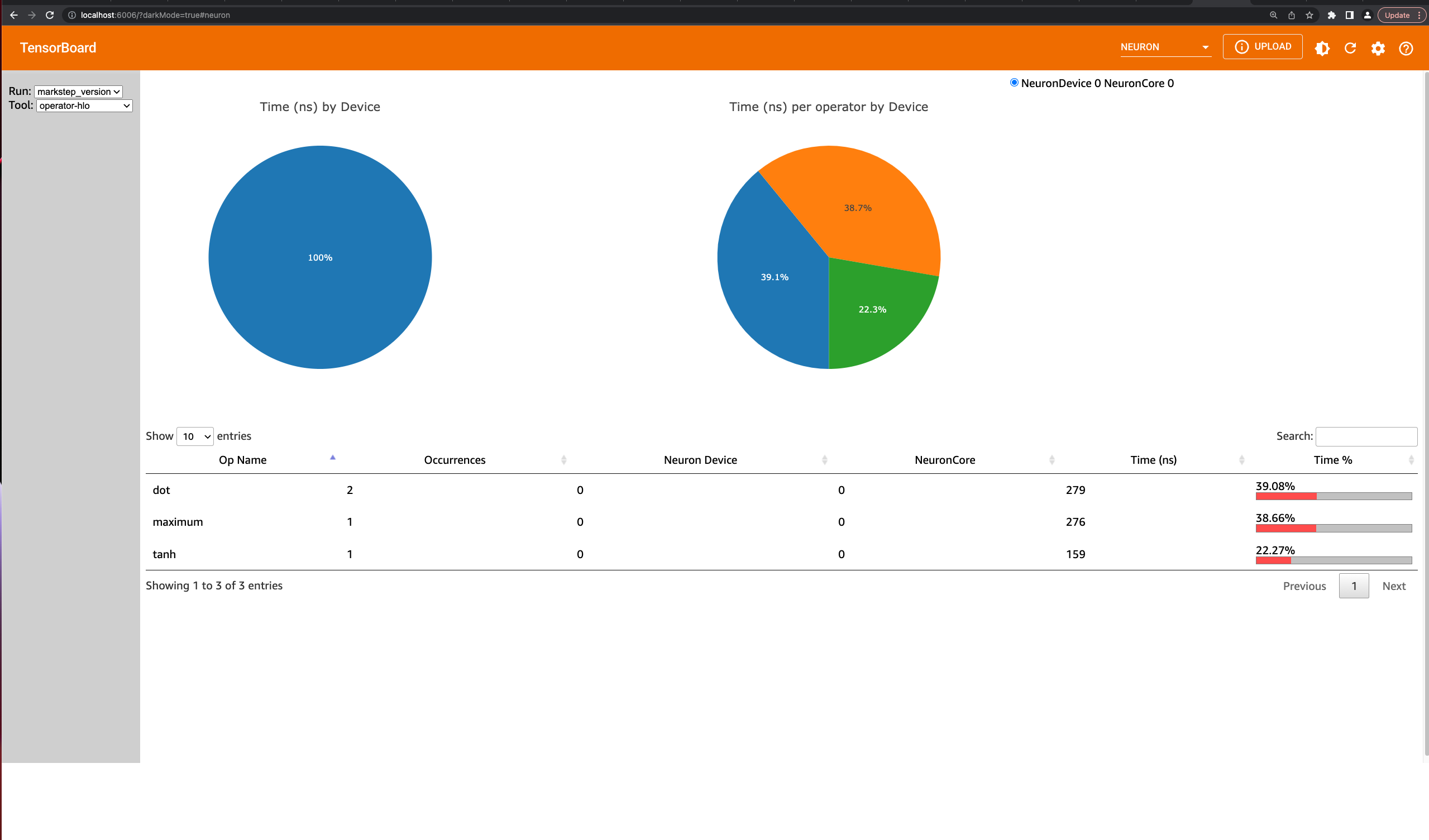
This view contains a pie-chart displaying the proportional execution time for each of the model operators on the hlo level for a Neuron device. The list of operators is shown in the bottom along with other details about number of occurrences, execution time and neuron device and core.

Note

For this simple model, the pie chart will be the same as the framework view. This won’t be the case for larger and more complex models.

Operator Trace View #

tensorboard-operator-trace-view

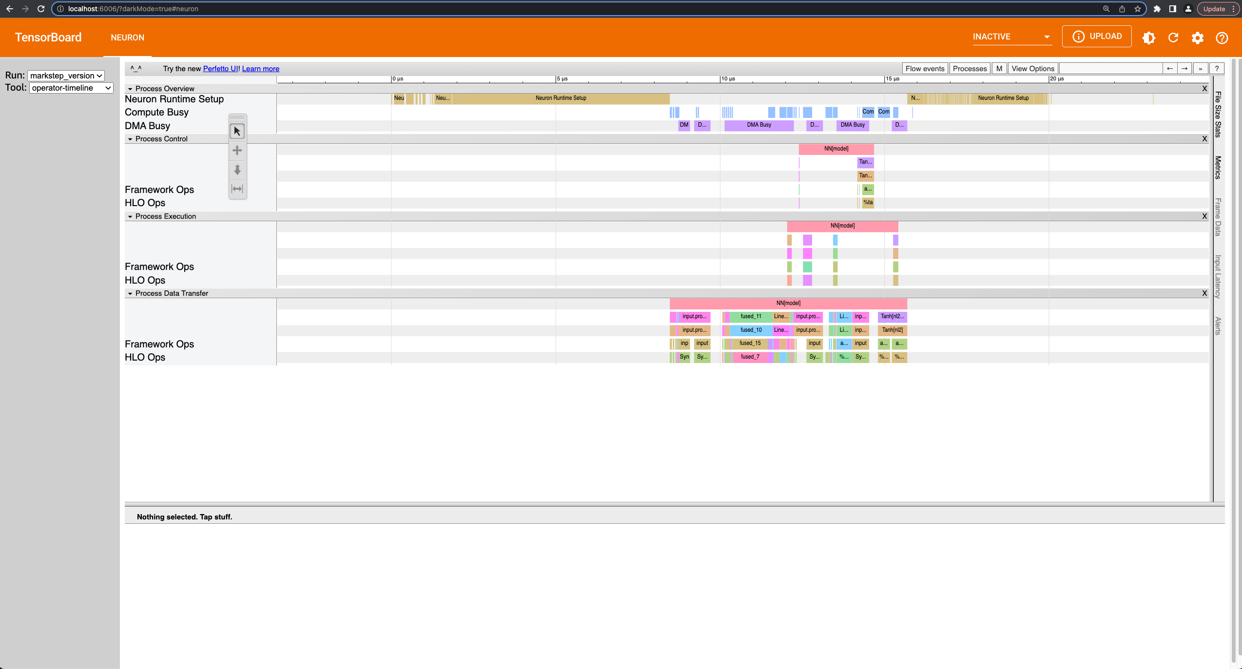
Trace View Sections#

Notice there are four sections: Process Overview, Control, Execution, and Data Transfer. In each section there are more subdivisions with each layer representing a certain level of abstraction. Also important to note that the timescale axis is aligned between the two sections. This is important to note as sometimes there are gaps in the process execution. Most of the time, there are data transfer operations happening in between the gaps.

Fusion Operators#

Simple Case: Zooming in on the operations, we can recognize some operations for a neural network, such as a dot product and transpose, but sometimes there will be fused operators (fusion operators). To understand these operators, click on it, and on the bottom of the dashboard, some information will appear.

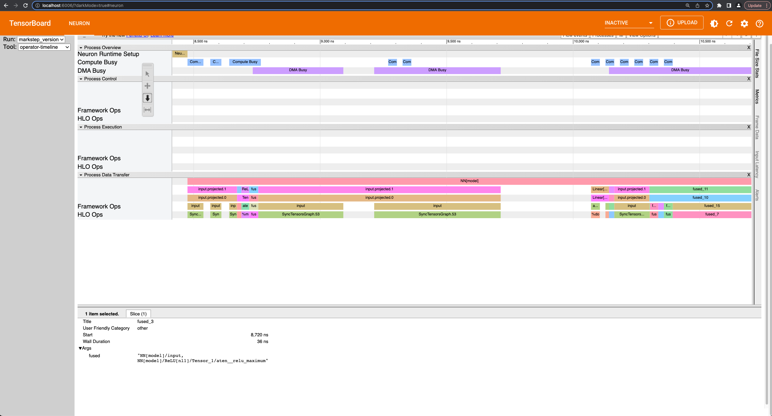
tensorboard-operator-trace-fusion-simple

Notice in the above example the fusion operator is fusing the operator before and after itself on the timeline. More specifically, fused_3 is a fusion of NN[model]/input and NN[model]/ReLU[nl1]/Tensor_1/aten__relu_maximum. These kinds of fusions occur when the neuronx-cc compiler has found an optimization relating to the two operators. Most often this would be the execution of the operators on separate compute engines or another form of parallelism.

Complex Case: Most often, the order of fusion operators can get a little complicated or contain “hidden” information. For the first example, let’s zoom into the data transfer section such that we see the timescale range from 6000 ns. to 6600 ns. It should look similar to below:

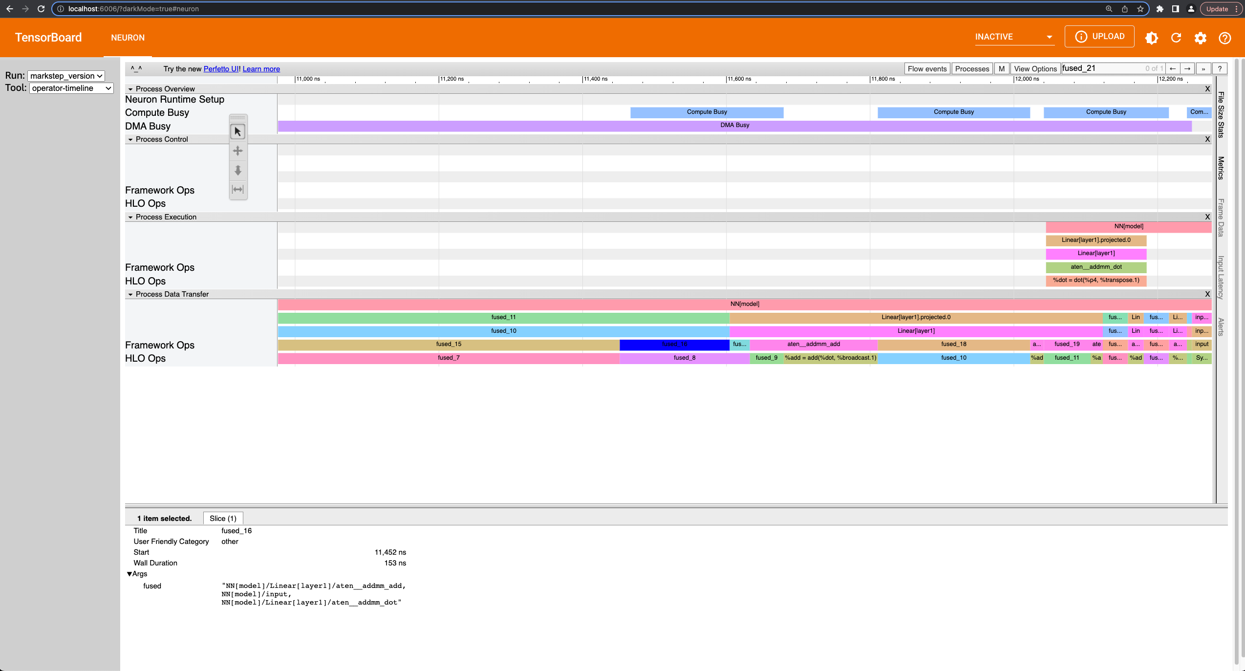
tensorboard-operator-trace-fusion-complex

Looking at fused_16 (11452 ns) we see it’s surrounded by other fused operators. Furthermore, the fused_16 operator fuses more than two operators: NN[model]/Linear[layer1]/aten__addmm_add, NN[model]/input, and NN[model]/Linear[layer1]/aten__addmm_dot. These operators can be found in the timeline, but sometimes the fused operators may not exist in the timeline due to it occurring within another operation. We go over an example of this case in Part 2.

Understanding the Low Level Timeline #

Looking at the trace we can look behind the scenes at how the model is executed on neuron hardware. Before proceeding with the analysis, it is worth recalling the way we defined the model for this tutorial:

class NN(torch.nn.Module):
   def __init__(self):
      super().__init__()

      self.layer1 = torch.nn.Linear(4,4)
      self.nl1 = torch.nn.ReLU()
      self.layer2 = torch.nn.Linear(4,2)
      self.nl2 = torch.nn.Tanh()

   def forward(self, x):
      x = self.nl1(self.layer1(x))
      return self.nl2(self.layer2(x))

Analysis#

Input Operators: We see input operators here. This is because in a markstep flow, we need to transfer inputs to the xla device. This is represented by the SyncTensorsGraph.53 call.

ReLU at the beginning: The first couple of blocks in the Process Data Transfer section initially appear to be confusing. There is an Input (0 ns.) block followed by a ReLU (100 ns.) operator. Under the hood here, ReLU is rewritten as an elementwise_max(arr,0), (0 here means an array with zeros) but to create this operation, the zeros have to be set in memory, which is a data operation. A general rule is that if an operator appears this early in the data transfer section, it most likely means there is an operation lowering involving setting some values into memory for use later on.

Memory allocation for Linear[layer1]: We resume with the data transfer operations. Here, memory is getting allocated for specific operators, and sometimes the allocated inputs get loaded onto operators while the rest of the input gets allocated. This can be seen at fused_18 (11811 ns.) and fused_23 (12181 ns.). Eventually the input gets fully allocated, and other allocations occur for dot products, transpose, and broadcast operators for Linear[layer1] and Linear[layer2].

Conclusion#

There are a few conclusions that can be determined from analyzing the timeline. We can see that we’ve been able to save a bit of time due to parallelism with fusion operations, and saving some compute time with preloading operations (ex. ReLU). A clear trend is that a majority of the time is spent on data transfer operations. It is also evident that even a simple Feed Forward NN becomes complicated when put under a microscope in the profiler. Facts such as the implementation of ReLU in the runtime/architecture, aren’t explicitly stated in the profiler, but do make themselves known by the unusual ordering placement of the trace blocks and unusual fusion operators.

In terms of action items that can be taken based on our narrative, there really isn’t any. This is a very very simple model that outputs after 8 microseconds, and we chose it because it is simple to understand. In more realistic examples we will aim to do more compute than data transfer on the hardware, and where possible to overlap data transfer and compute between sequential operations.

The profiler revealed a lot of optimizations that were done, via fusion operators and parallelism. However, the end goal of this tool is to be able to improve performance by revealing the bottlenecks of the model.

Note

While we did explain some of the quirks visible in the profiler at a microscopic level, it isn’t necessary to do so for normal use. This tutorial introduced the microscopic explanation for these occurrences to show to the user that this is indeed what happens in the hardware when executing a simple FFNN.

Part 2: Operator Level Trace with `torch_neuronx.trace()` workflow #

Set Up #

The setup will be similar to Part 1.

cd ~/neuron_profiling_tensorboard_examples
mkdir tutorial_2
cd tutorial_2

# this is where our code will be written
touch run.py

Here is the code for run.py:

import os
import time
import torch
import torch_neuronx
from torch_neuronx.experimental import profiler

class NN(torch.nn.Module):
   def __init__(self):
      super().__init__()

      self.layer1 = torch.nn.Linear(4,4)
      self.nl1 = torch.nn.ReLU()
      self.layer2 = torch.nn.Linear(4,2)
      self.nl2 = torch.nn.Tanh()

   def forward(self, x):
      x = self.nl1(self.layer1(x))
      return self.nl2(self.layer2(x))

model = NN()
model.eval()

inp = torch.rand(4,4)

output = model(inp)

with torch_neuronx.experimental.profiler.profile(
   port=9012,
   profile_type='operator',
   ms_duration=10000,
   traced_only=True):

   neuron_model = torch_neuronx.trace(model,inp,compiler_workdir="./compiler_cache")
   neuron_model(inp)

print("==CPU OUTPUT==")
print(output)
print()
print("==INF2 OUTPUT==")
print(output_neuron)

Important code differences from Part 1 #

import torch_xla.core.xla_model as xm is no longer necessary
Set traced_only=True in torch_neuronx.experimental.profiler.profile(). This option is necessary for traced models, otherwise the generated profile will not be accurate or not work.
Tracing the model with torch_neuronx.trace() and removing xm.markstep().

Otherwise, the code is the same as Part 1.

Running Part 2 #

To Run:

python run.py

The output will look almost identical as Part 1

Loading the Operators Level Trace in TensorBoard #

Run tensorboard --load_fast=false --logdir logs/, just like Part 1.

Note

Check Viewing the Trace on TensorBoard to understand TensorBoard interface

Timeline View:

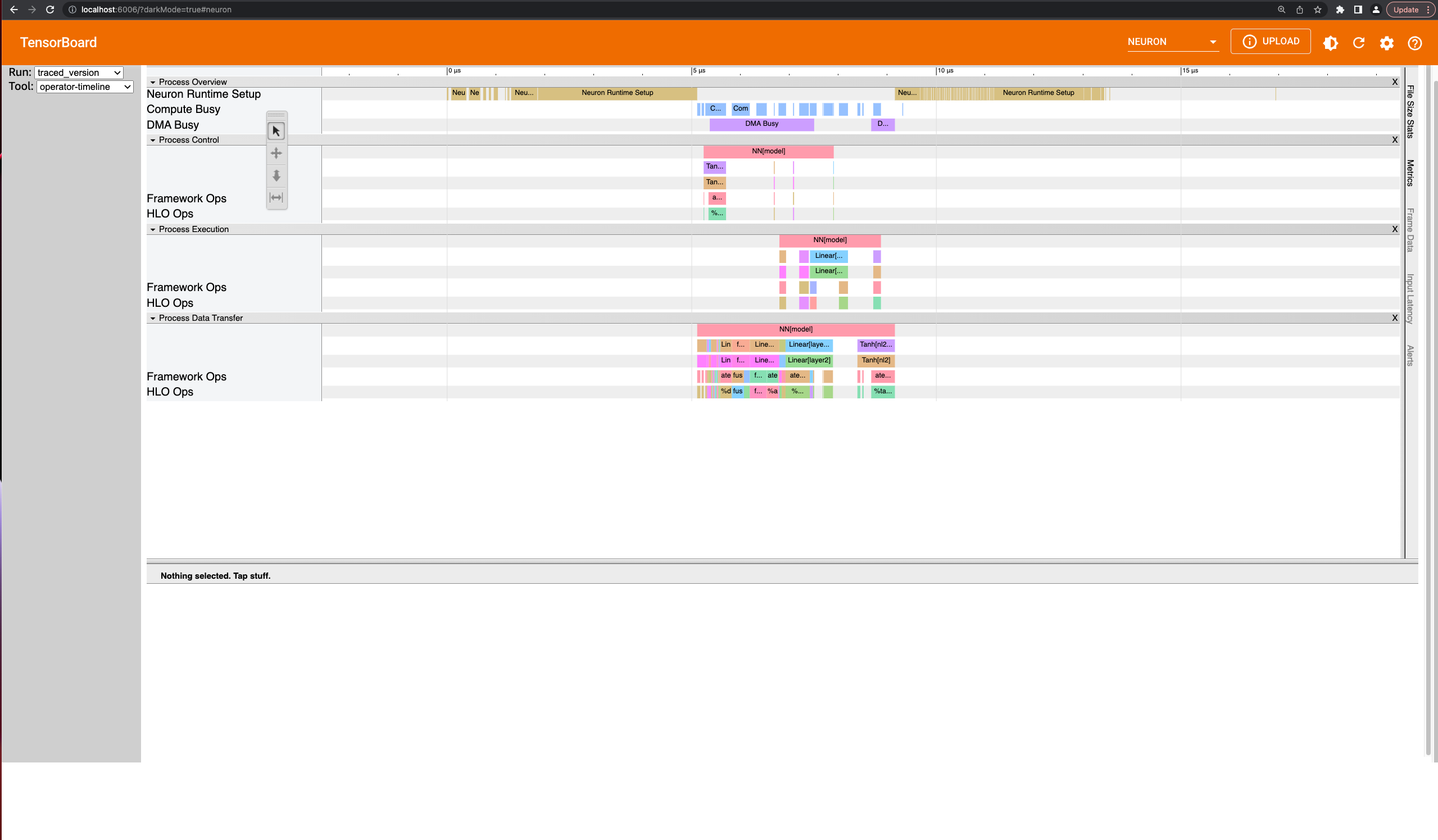
tensorboard-operator-trace-view-traced

Notable Differences in Timeline View from Part 1:#

No Input Operators: For a traced model, we do not transfer the input to an xla device, so these operations are not seen on the timeline. This also affects scheduling, which is why the time taken in the profiling is less than the markstep one.

Combined Loading of Linear[layer1] and Tanh: fused_19 (5824 ns) contains a fusion between Linear[layer1] and Tanh[nl2]. This might be a bit odd, but such data loading parallelism can be understood by understanding how tanh is implemented. Typically, functions like tanh are implemented by lookup tables that require being pre-loaded onto memory, which is a data transfer operation. A bulk of data transfer operations are done in the beginning to optimize computations.

Note

Despite these differences, the big picture conclusion drawn from Part 1 still holds, as the two timelines are more similar than different. Some new insights drawn is that the traced model performs better than the markstep flow, since this was profiling a single forward pass.

This document is relevant for: Inf1, Inf2, Trn1, Trn1n

AWS Neuron Documentation

Profiling PyTorch Neuron (torch-neuronx) with TensorBoard

Contents

Profiling PyTorch Neuron (`torch-neuronx`) with TensorBoard#

Introduction #

Setup #

Prerequisites #

Environment #

Part 1: Operator Level Trace for `xm.markstep()` workflow #

Goal #

Set Up #

Understanding the Code #

Running The Profiler #

Loading the Operators Level Trace in TensorBoard #

Operator Framework View #

Operator HLO View #

Operator Trace View #

Trace View Sections#

Fusion Operators#

Understanding the Low Level Timeline #

Analysis#

Conclusion#

Part 2: Operator Level Trace with `torch_neuronx.trace()` workflow #

Set Up #

Important code differences from Part 1 #

Running Part 2 #

Loading the Operators Level Trace in TensorBoard #

Notable Differences in Timeline View from Part 1:#

AWS Neuron Documentation

Profiling PyTorch Neuron (torch-neuronx) with TensorBoard

Contents

Profiling PyTorch Neuron (torch-neuronx) with TensorBoard#

Trace View Sections#

Fusion Operators#

Analysis#

Conclusion#

Profiling PyTorch Neuron (`torch-neuronx`) with TensorBoard#