Trainium3 Architecture Guide for NKI

Note

If nisa API is mentioned for a given architectural feature, that means NKI support is ready yet.

In this guide, we will dive into hardware architecture of fourth-generation NeuronDevices: Trainium3. This guide will highlight major architectural updates compared to the previous generation (Trainium2). Therefore, we assume readers are familiar with Trainium/Inferentia2 Architecture Guide and Trainium2 Architecture Guide for NKI to understand the basics of NeuronDevice Architecture.

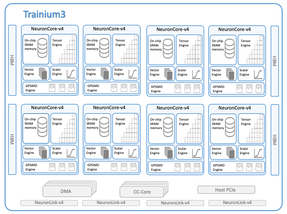
The diagram below shows a block diagram of a Trainium3 device, which consists of:

• 8 NeuronCores (v4).

• 4 HBM stacks with a total device memory capacity of 144 GiB and bandwidth of 4.7 TB/s.

• 128 DMA (Direct Memory Access) engines to move data within and across devices.

• 20 CC-Cores for collective communication.

• 4 NeuronLink-v4 for device-to-device collective communication.

The rest of this guide discusses NeuronCore-v4’s major architectural updates compared to NeuronCore-v3 that are relevant for NKI programmers.

NeuronCore-v4 Compute Engine Updates

The figure below is a simplified NeuronCore-v4 diagram of the compute engines and their connectivity to the two on-chip SRAMs, which are SBUF and PSUM. This is similar to previous versions of NeuronCore.

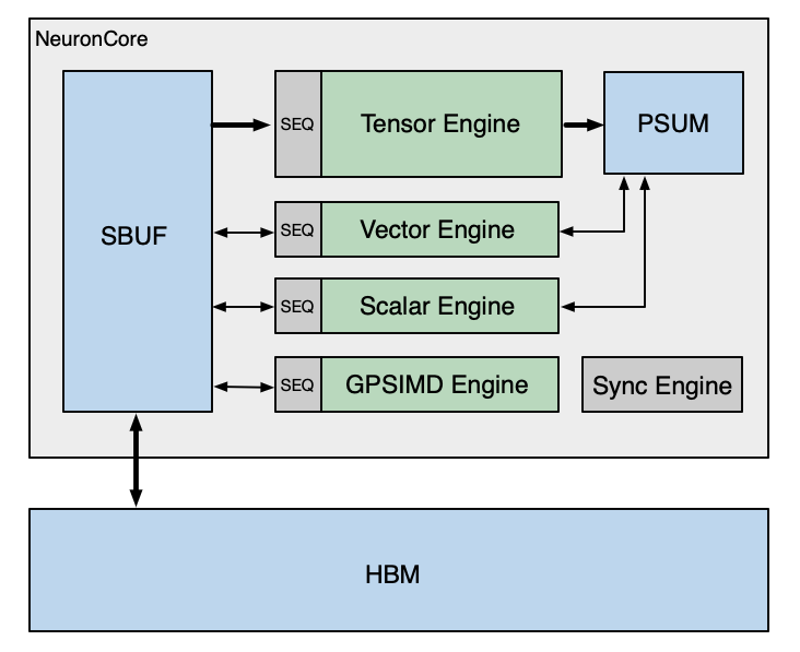
The NeuronCore-v4 SBUF capacity is 32MiB (up from 28 MiB in NeuronCore-v3), while the PSUM capacity remains the same at 2MiB. The engine data-path widths and frequencies are updated to the following:

Table 10 Compute Engine Specifications

Device Architecture	Compute Engine	Data-path Width (elements/cycle)	Frequency (GHz)
Trainium3	Tensor	8x128 (MXFP8 dense input) or 2x128 (non-MXFP8 dense input) or 5x128 (sparse input); 1x128 (output)	2.4
	Vector	512 BF16/FP16/FP8 input/output; 256 input/output for other data types	1.2
	Scalar	256 BF16/FP16/FP8 input/output; 128 input/output for other data types	1.2
	GpSimd	128 input/output for all data types	1.2

Sync Engine has not changed since previous Trainium architectures. Next, we will go over major architectural updates to each compute engine.

Tensor Engine

Tensor Engine is optimized for tensor computations such as GEMM, CONV, and Transpose. A NeuronCore-v4 Tensor Engine delivers 315 MXFP8/MXFP4 TFLOPS, where MXFP8/MXFP4 are OCP (Open Compute Project) compliant data type formats. Besides quantized data types, a NeuronCore-v4 Tensor Engine also delivers 79 BF16/FP16/TF32 and 20 FP32 TFLOPS of tensor computations. The rest of this section describes new architectural features introduced in the NeuronCore-v4 Tensor Engine.

Quad-MXFP8/MXFP4 Matmul Performance

The NeuronCore-v4 Tensor Engine (TensorE) supports two new input data types: MXFP8 and MXFP4, where MX stands for “microscaling”, as defined in the OCP standard. Microscaling is a subset of absmax (absolute maximum quantization), where quantization scale factors are calculated using absolute maxima of fine-granularity groups of values, as opposed to having tensor- or channel-wise scale factors. It can significantly improve the amount of information preserved in the quantized values. The supported scaling group size is 32: That means that 32 MXFP8/MXFP4 elements along the matrix multiplication (matmul) contraction dimension share the same 8-bit MX scale value. The Tensor Engine performs matrix multiplications of MXFP8 or MXFP4 input matrices [1] and dequantization with the MX scales in a single instruction, with the output either in FP32 or BF16. We will refer to MXFP8 and MXFP4 matmul as MX matmul in the rest of this guide. An MX matmul with either the MXFP8 or MXFP4 datatype runs at 4x the throughput compared to a BF16/FP16 matmul.

[1]

Multiplying an MXFP8 matrix with an MXFP4 matrix is also allowed.

Logically, TensorE quadruples the MX matmul performance, as compared to BF16 performance, by quadrupling the maximum contraction dimension of the matmul instruction from 128 (for BF16/FP16) to 512, effectively presenting a 512x128 systolic array to the programmer. Under the hood, since the systolic array is still organized as a grid of 128x128 processing elements, each processing element performs four pairs of MX multiplications and also accumulation of the four multiplication results per cycle. This is similar to the Double-FP8 performance mode in the Trainium2 TensorE (discussed in Trainium2 Architecture Guide), but the data layout requirements for MX matmul are distinct and discussed as below.

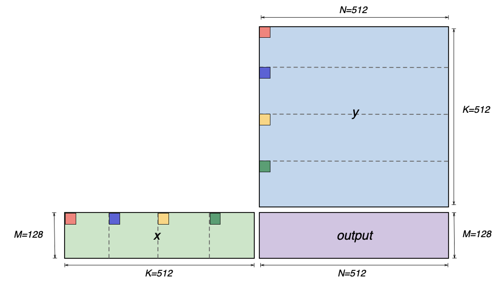
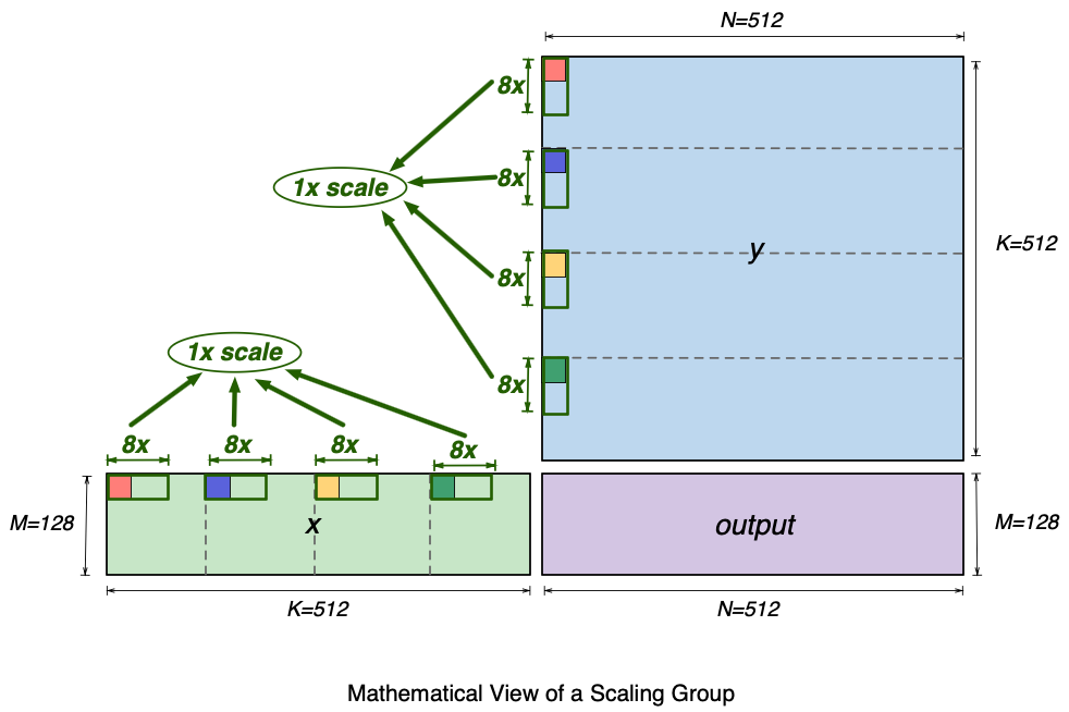
Mathematically, an MX matmul instruction can perform a multiplication of an 128x512 matrix and a 512x512 matrix (that is, MxKxN matmul, M=128, K=512, N=512). The figure below shows a visualization of the two input matrices (x and y) and the matmul output matrix (output). The figure also highlights four elements (red, blue, yellow and green) in the first row of the x matrix and in the first column of the y matrix. These four elements are 128 (K//4) elements apart within the row and column. Each pair of same-colored elements from x and y matrices will get multiplied, and the multiplication results are subsequently accumulated in the matmul operation, inside the TensorE. We will use these elements to illustrate the SBUF layout requirements for these matrices next.

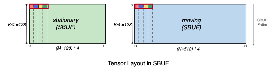
The figure below shows how the above matrices should be laid out in SBUF in preparation for MX matmul. For visualization purposes, the x matrix is rotated 90 degrees, such that the contraction K dimension is aligned with the SBUF partition dimension. In addition, we pack the four highlighted elements that used to be 128 elements apart back-to-back along the free dimension. As a result, the matmul contraction dimension K=512 is split into two dimensions: (1) the partition dimension of size 128 and (2) the most minor (fastest) free dimension of size 4. The y (moving) matrix follows a similar four-element packing pattern along the free dimension. The MX matmul instruction requires that data is packed in such quads of elements. In NKI, programmers can directly work with MX data using special quad (x4) packed data types: float8_e5m2_x4, float8_e4m3fn_x4, and float4_e2m1fn_x4.

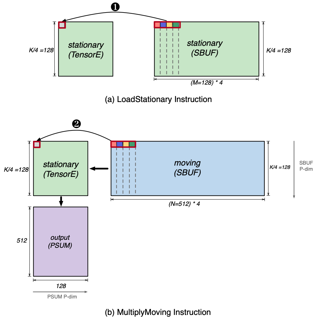
Next, we invoke the LoadStationary and MultiplyMoving instructions to perform the matrix multiplications using the above tensors in SBUF. This is illustrated in the figure below. The LoadStationary instruction loads the MX stationary tensor (K/4=128, M=128, 4) into TensorE, which stores four MX data elements into a single processing element as shown in ❶. Next, the MultiplyMoving instruction streams the moving tensor horizontally across the loaded stationary tensor. Similar to LoadStationary, four elements of moving tensor are sent to the same processing element simultaneously as shown in ❷, such that they can get multiplied with the corresponding loaded stationary elements.

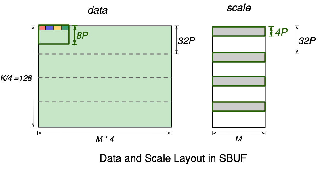
Since MX matmul in TensorE performs dequantization in addition to the multiplication of the input matrices, we discuss how the scale tensor is laid out in SBUF for TensorE consumption. Recall that the supported MX group size on NeuronCore-v4 TensorE is 32 elements along the contraction dimension. Each input MX matrix to the matmul operation therefore has its own scale tensor. In fact, the highlighted x4 elements within each matrix in the above images are within the same scaling group. The diagram below shows the full 32-element scaling group that includes these highlighted x4 elements within matrix x and y.

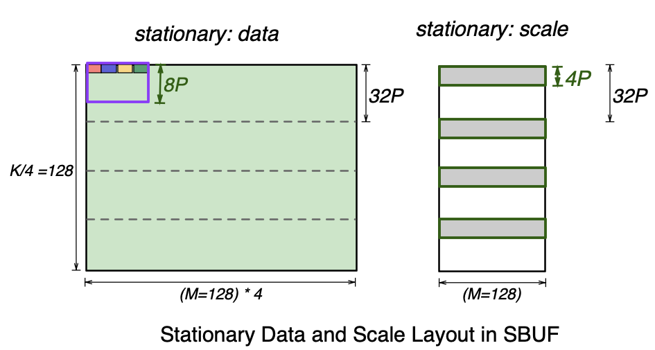
Let’s focus on the stationary data and scale tensor layout below. On the left, the purple rectangle represents the 32-element scaling group that includes the four highlighted elements, which spans 8 SBUF partitions (8P) and 4 elements per partition.

A single scaling group corresponds to one 8-bit integer scale. Therefore, for every 32 partitions of the data tensor, we get 32/8=4 partitions worth of scale factors. As shown in the scale tensor below, the full scale tensor is split across four SBUF quadrants, where each quadrant holds 4 partitions worth of scales. Note the free dimension of the scale tensor is M=128, which is 4x smaller than the data tensor. This is because the four packed colored elements in the data tensor belong to the same scaling group and hence share a single scale. Within each SBUF quadrant, 32-4=28 partitions are unused in the scale tensor below. Multiple scale tensors for different MX matmul instructions can be packed together to fill up the unused partitions. See NKI tutorial for more discussion on working with scale tensors.

The moving data and scale tensor layout follows the same rules. Therefore, an MX matmul on TensorE requires four input tensors:

1. stationary data

2. stationary scale

3. moving data

4. moving scale

In NKI, programmers can define MX data tensors using the special x4 data types. The maximum tile size for stationary MX data tensor is [128, 128] in x4 data types ([128, 512] of actual values), while the maximum tile size for moving MX data tensor is [128, 512] in x4 data types ([128, 2048] of actual values). One convenience of the x4 datatypes is that the output matrix dimensions map directly to the sizes of the free dimensions of the input matrices. Similarly, the maximum tile size for stationary and moving MX scale tensors are [128, 128] and [128, 512] in nl.uint8, respectively. The API to invoke an MX matmul is:

nisa.nc_matmul_mx(moving, stationary, moving_scale, stationary_scale)

BF16 Matmul Results in PSUM

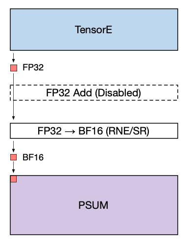
Prior to the NeuronCore-v4, the Tensor Engine always passes FP32 matrix multiplication results to PSUM unless transpose mode is turned on. Similarly, the PSUM buffer was restricted to FP32 near-memory accumulation (fp32_psum_tensor += fp32_matmul_output). Starting with the NeuronCore-v4, the Tensor Engine allows the matrix multiplication instruction (nisa.nc_matmul) to store BF16 data into the PSUM buffer directly and also to perform addition to a BF16 tensor stored in PSUM.

NKI programmers can use this feature through the existing nisa.nc_matmul API:

psum_tensor = nl.ndarray((128, 512), dtype=nl.bfloat16, buffer=nl.psum)

nisa.nc_matmul(..., dst=psum_tensor, psum_accumulate_flags=1)
nisa.nc_matmul(..., dst=psum_tensor, psum_accumulate_flags=0)

Note that the accumulation performed during a matmul operation within the systolic array is still performed using FP32 data. When writing the matmul results into a BF16 PSUM tensor location, the downcast from FP32 to BF16 is performed immediately before the write. The downcast can use the RNE (round nearest even) or SR (stochastic rounding) mode. The figure below illustrates this data flow.

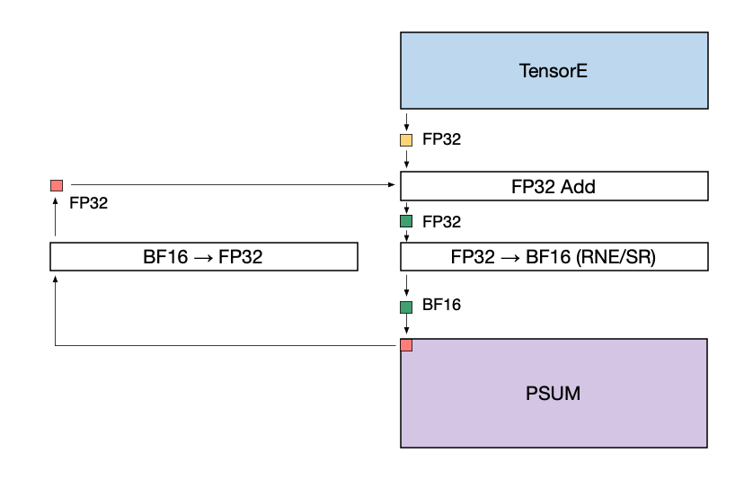
When adding the matmul results to an existing BF16 tensor stored in PSUM the following operations are performed:

• The existing PSUM tensor (red) is upcast to FP32.

• The PSUM tensor (now in FP32) and the TensorE output (yellow) are added together at FP32 precision.

• The result of the addition (green) is converted to BF16 using the given rounding mode, and written back to PSUM.

Background Transpose

The NeuronCore-v4 TensorEngine supports a new background transpose functionality, which allows it to run a transpose operation in parallel to another matrix multiplication (or another transpose). It allows us to achieve close to double performance on long chains of transposes, or to overlap a larger matrix multiplication with transpose operations in the background.

NKI programmers are not required to enable background transpose explicitly to leverage the performance improvements from this feature. The decision to trigger background transpose is made automatically by the hardware.

Vector Engine

The Vector Engine is optimized for vector computations, in which every element of the output is dependent on multiple input elements. Examples include the axpi operations (Z=aX+Y), Layer Normalization, and Pooling operations. The NeuronCore-v4 Vector Engine delivers a total of 1.2 TFLOPS of FP32 computations and can handle various input/output data-types, including FP8, FP16, BF16, TF32, FP32, INT8, INT16, and INT32. The rest of this section describes new architectural features introduced in the NeuronCore-v4 Vector Engine.

MX data-type Quantization

The NeuronCore-v4 VectorE supports quantizing FP16/BF16 data to MXFP8 tensors (both data and scales) in a layout that TensorE can directly consume for MX matmul, as described in the Quad-MXFP8/MXFP4 Matmul Performance section above. As a reminder, an MxK MXFP8 matrix, where K is the contraction dimension, requires the following data and scale layout in SBUF:

The VectorE can natively quantize BF16/FP16 data to produce this layout using the QuantizeMX instruction. QuantizeMX calculates the required scales for each group of 32 values, divides them by the calculated scale, and casts to the target MXFP8 datatype (as per the OCP specification):

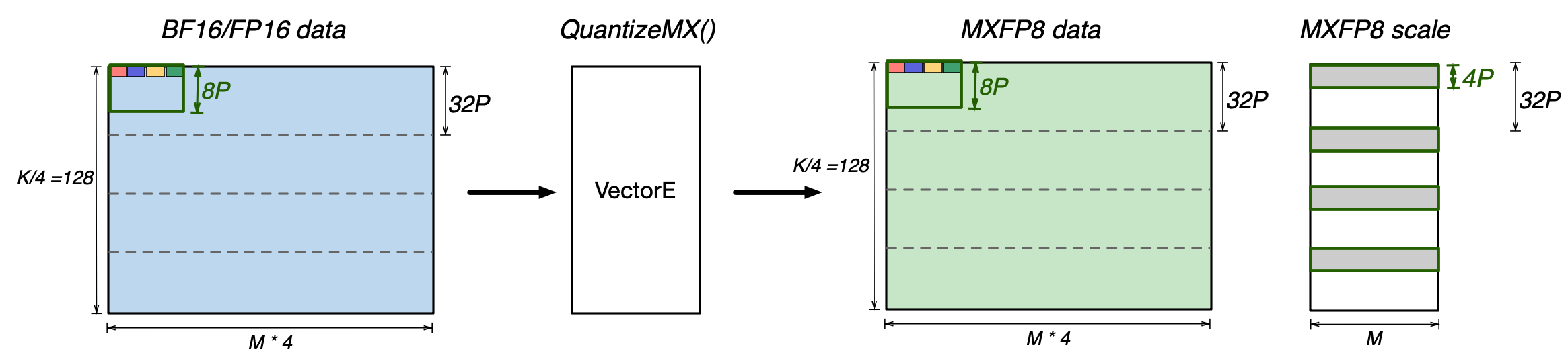
The source FP16/BF16 data must be in SBUF, and has to be in a layout that exactly matches the target MXFP8 data layout (QuantizeMX preserves the data layout). The target MXFP8 data and scales also have to be in SBUF. The quantization instruction can quantize four input elements per partition, per cycle (i.e., 4x Vector performance mode).

In NKI, programmers can perform such an MX data type quantization using the nisa.quantize_mx API.

Fast Exponential Evaluation

The NeuronCore-v4 Vector Engine introduces a new instruction to perform fast exponential evaluation (nisa.exponential(dst=out_tile, src=in_tile, …)), at 4x the throughput compared to the nisa.activation(op=nl.exp) instruction on the Scalar Engine. In addition to the exponential function, the instruction on Vector Engine can also apply a subtraction before the exponential function and an accumulation after:

# Inputs:
# src tile [M, N]
# row_max tile [M, 1]
# Outputs:
# dst tile of the same shape [M, N]
# row_sum tile [M, 1]
for i in range(M): # parallel (partition) dimension
    row_max[i, 0] = 0
    for j in range(N): # sequential (free) dimension
        dst[i, j] = exp(src[i, j] - row_max[i, 0])
        row_max[i, 0] += dst[i, j]

This particular pattern is useful to speed up the Softmax operator, which is commonly on the critical path of long context length self-attention in large language models (LLMs):

\[Softmax(X)=\frac{e^{X_i-max(X)}}{\sum_i e^{X_i-max(X)}}\]

X is a vector of attention scores in the context of self-attention, which corresponds to a row in the src tile in the above instruction pseudo code.

XORWOW-based PRNG

The NeuronCore-v4 VectorE provides hardware support to produce PRNG (pseudo-random) values using XORWOW as the underlying algorithm. Compared to the LFSR-based algorithm used in VectorE prior to NeuronCore-v4, XORWOW produces higher quality random values. The NeuronCore-v4 VectorE can produce 4x 32-bit PRNG values per compute lane per engine cycle.

In addition, the NeuronCore-v4 VectorE introduces support for loading and storing XORWOW random states from and to SBUF (or PSUM), across all 128 compute lanes. Within each compute lane, four XORWOW random states are tracked to maintain the nisa.rand2() instruction throughput, with each state comprising 6 uint32 values. For more details, refer to the nisa.rand_set_state and nisa.rand_get_state API documentation. This new state load/store capability in NeuronCore-v4 VectorE, which was not available in previous NeuronCore versions, allows users to save and restore random states for reproducible training runs more easily.

Scalar Engine

The Scalar Engine is optimized for scalar computations in which every element of the output is dependent on one element of the input. The NeuronCore-v4 Scalar Engine delivers a total of 1.2 TFLOPS of FP32 computations and can support various input/output data types, including FP8, FP16, BF16, TF32, FP32, INT8, INT16, and INT32. The rest of this section describes new architectural features introduced in the NeuronCore-v4 Scalar Engine.

Performance mode

The Trainium3 ScalarE now natively supports the tensor_scalar and tensor_copy instructions (same as VectorE), and offers up to 2x performance uplift for BF16/FP16 datatypes, which is the same as the 2x performance mode on VectorE introduced with Trainium2. For those instructions, NKI users are able to select the execution engine, which can help offload either one of the engines, or load balance between them, depending on workload characteristics.

More flexible nisa.activation

Trainium3 introduces the Activation2 instruction, which provides more flexibility to users compared to the existing Activation instruction. Unlike Activation, which only supports the combination of scale multiplication and bias addition, Activation2 supports bias subtraction and allows users to disable scale multiplication and bias addition entirely. Further, while Activation only supported add as a reduce command, Activation2 supports add, max, min, absmax, and absmin reductions.

Data Movement and DMA updates

SBUF/PSUM indirect access

The NeuronCore-v4 SBUF/PSUM introduce a new indirect addressing mode for all compute engines (TensorE/VectorE/ScalarE/GpsimdE), which allows gathering or scattering SBUF and PSUM tensors along the free (F) dimension. Consider a tensor of shape [128, 512] located in SBUF, which occupies 128 partitions with 512 elements per partition. Suppose a user is interested in only accessing the elements 0, 128 and 384 along the free dimension across all 128 partitions for a single computation operation, such as nisa.nc_matmul:

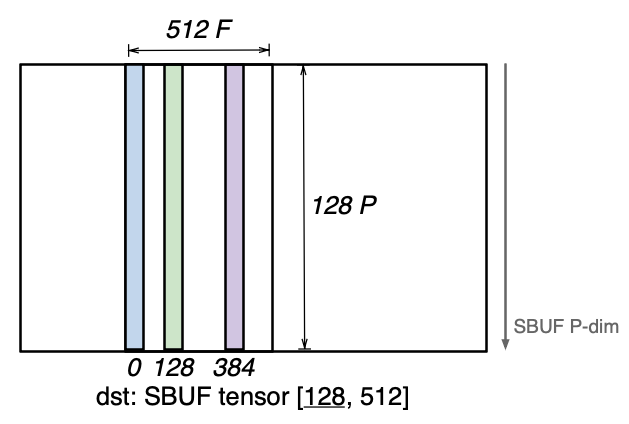
Since these three vectors do not have a uniform stride along the free dimension; the access pattern is not a tensorized pattern (i.e. a regular N-dimensional access pattern). Prior to NeuronCore-v4, such an access pattern would require three separate instructions (such as nisa.nc_matmul) to perform the computation on all three vectors.

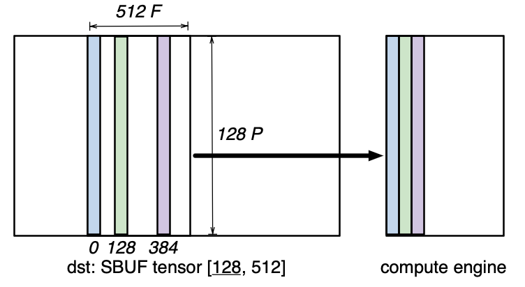
In NeuronCore-v4, all compute engines can perform a gather access pattern to directly access those three vectors in a single instruction:

Similarly, an indirect scatter operation allows any engine to scatter a set of vectors into a target tensor:

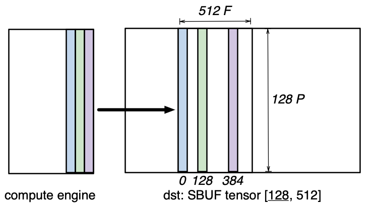
Both styles of indirection use a separate offset tensor to encode which vectors to access.

SBUF Read-Add-Write

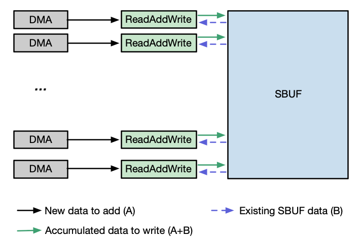
NeuronCore-v4 introduces an enhanced SBUF capability that enables on-the-fly tensor accumulation near memory. This feature allows DMA engines to perform B+=A operations, where tensor B resides in SBUF and tensor A can be sourced from any accessible memory location (such as HBM or SBUF). Tensors A and B can be either BF16 or FP32 data types, but they must have a matching data type within a single DMA transfer performing the Read-Add-Write operation. This near-memory accumulation maintains the same throughput as standard DMA copy operations to SBUF (compared to 50% DMA throughput via DMA collective compute engines prior to NeuronCore-v4), enabling efficient in-place tensor updates without additional memory overhead.

The figure below illustrates the data flow that is used to enable this SBUF accumulation feature. As the first, a DMA unit transfers tensor A to the ReadAddWrite unit adjacent to the SBUF. The ReadAddWrite unit then retrieves tensor B from SBUF, performs the addition of A and B, and writes the result back to tensor B’s original location in SBUF.

Trainium3 DMA engines support Traffic Shaping, which enables configurable bandwidth allocation across different DMA operations. The DMA Traffic Shaping feature supports 4 distinct classes of service, enabling fine-grained control over the priorities of data movement. This capability is particular beneficial when optimizing parallel computation and communcation (collevives operations) across multiple NeuronCores.

DMA QoS

The Trainium3 DMA engines support QoS (quality-of-service), configured per DMA queue through user registers. Note that this implementation of QoS uses a “strict priority”: the transfers in a DMA queue with the highest priority are always scheduled first, before any other DMA queues are serviced. This DMA queue-based QoS feature is particularly useful in the context of parallelizing computation and communication (collectives operation) among multiple NeuronCores.