Introduction to NKI Kernel Optimization#
The Neuron Kernel Interface (NKI) provides an API for writing hand-tuned kernels. You use the Instruction Set Architecture (ISA) of a Neuron device directly to speed up critical parts of an ML model. This topic covers how you develop and tune NKI kernels and how this applies to developing with the AWS Neuron SDK. The Neuron Profiler helps you identify opportunities to improve ML model performance and drive hand-tuned optimizations with a NKI kernel.
Overview#
Developers commonly create NKI kernels to accelerate critical operations in larger ML inference or training models. Just as you might accelerate a traditional program by writing small parts in inline assembler, NKI lets you directly program the underlying Neuron hardware using the same ISA instructions the Neuron Compiler generates. In this overview, we use a kernel that performs matrix multiply as an example. We use the profiler to work from a simpler, more obviously correct version of the kernel to a version that performs better by improving memory usage by removing redudant loads and increasing DMA efficiency through blocking which better overlaps loading data and computing results. Along the way, we use a test program in PyTorch or JAX to ensure each step preserves a working kernel. We use the Neuron Explorer to drive additional performance improvements. We also change the kernel from being memory bound in the initial tiled implementation to being compute bound, as we would expect, in the optimized version of the kernel.
Applies to#
This concept is applicable to:
Improving the performance of critical sections of ML inference or training models.
Writing small performant kernels for standalone ML inference or training.
When to write a kernel?#
The Neuron Compiler takes ML models written in PyTorch, JAX, and other frameworks and generates the best performing code it can based on that model. Like any general purpose compiler, it may make optimization decisions that work well for the general case but may not produce optimal code for this specific model. The Neuron Kernel Interface (NKI) provides a mechanism for replacing sections of a model with a hand-tuned kernel. The first step in identifying a good candidate for turning a section of a model into a kernel is the Neuron Profiler, which provides a view on how the model performs.
The Neuron Profiler can help indicate where the model might benefit from optimization. You can map sections in the Neuron Profiler where one or more engines are idle while waiting on DMA or similar apparent gaps to places in the model where code may execute several times. These can be good candidates for writing a custom kernel. Good candidates are similar to where you might split a large function into smaller functions in a traditional program. This means some “minimum cut” in the graph where there are relatively few inputs and outputs of the kernel.
Starting simple#
The end goal of writing a kernel is to improve the performance of the model, but the first step is to write a kernel that correctly performs the operation you wish to replace in the graph. As a motivating example, suppose that the section of the graph you wish to replace consists of a matrix multiply of two relatively large matrices. Kernels will often be more sophisticated than this, as you can see by looking at the Neuron Kernel Library (NKL), for instance performing functions like RMSNorm-Quant or QKV, but matrix multiply may be an aspect of these more sophisticated kernels.
NKI provides the nki.isa.nc_matmul instruction to perform a matrix multiply. This instruction operates over a restricted sized matrix with at most a 128 x 128 “stationary” (weights) matrix and a 128 x 512 “moving” (ifmap) matrix. This allows you to produce a 128 x 512 matrix, at most, as output. The “stationary” matrix must be transposed to get a result that is not transposed. To call the nki.isa.nc_matmul instruction, provide to the state buffer (SBUF), and the result will be written into the partial sum buffer (PSUM). If you use a small driver program to invoke the kernel, the arguments will be passed in from the device memory (HBM) and the result will be read from HBM as well. The kernel will move inputs from HBM to SBUF, call the nki.isa.nc_matmul instruction, move the result from PSUM to SBUF (you cannot move data directly from PSUM to HBM), and then from SBUF to HBM.
import nki
import nki.language as nl
import nki.isa as nisa

@nki.jit(platform_target="trn2")
def matrix_multiply_kernel(lhsT, rhs):
  """NKI kernel to compute a matrix multiplication operation on a single tile

  Args:
    lhsT: an input tensor of shape [K,M], where both K and M are, at most,
      128.  It is the left-hand-side argument of the matrix multiplication,
      delivered transposed for optimal performance.
    rhs: an input tensor of shape [K,N], where K is, at most, 128, and N
      is, at most, 512.  It is the right-hand-side argument of the matrix
      multiplication.
  Returns:
    result: the resulting output tensor of shape [M,N]
  """
  # Verify that the lhsT and rhs are the expected sizes.
  K, M = lhsT.shape
  K_, N = rhs.shape

  # Ensure that the contraction dimension matches
  assert K == K_, \
    f"Contraction demention {K} does not match {K_}, did you remember to transpose?"

  # Ensure the dimensions will fit within the constrins of matmul.
  assert K <= nl.tile_size.pmax, \
    f"Expected partition dimension in lhsT ({K}) to be less than {nl.tile_size.pmax}"
  assert M <= nl.tile_size.gemm_stationary_fmax, \
    f"Expected free dimension in lhsT ({M}) to be less than " \
    f"{nl.tile_size.gemm_stationary_fmax}"
  assert N <= nl.tile_size.gemm_moving_fmax, \
    f"Expected free dimension in rhs ({N}) to be less than " \
    f"{nl.tile_size.gemm_moving_fmax}"

  # Allocate tiles for lhsT and rhs on sbuf (uninitialized)
  lhsT_tile = nl.ndarray(shape=lhsT.shape, dtype=lhsT.dtype, buffer=nl.sbuf)
  rhs_tile = nl.ndarray(shape=rhs.shape, dtype=rhs.dtype, buffer=nl.sbuf)

  # Copy the input matrices from HBM to SBUF
  nisa.dma_copy(dst=lhsT_tile, src=lhsT)
  nisa.dma_copy(dst=rhs_tile, src=rhs)

  # Perform matrix multiply, result will be written into PSUM
  result_tile = nl.ndarray(shape=(M, N), dtype=nl.float32, buffer=nl.psum)
  nisa.nc_matmul(dst=result_tile, stationary=lhsT_tile, moving=rhs_tile)

  # Copy result to SBUF (we cannot copy directly from PSUM to HBM)
  result_tmp = nl.ndarray(shape=result_tile.shape,
                          dtype=result_tile.dtype,
                          buffer=nl.sbuf)
  nisa.tensor_copy(dst=result_tmp, src=result_tile)

  # Copy result to HBM
  result = nl.ndarray(shape=result_tmp.shape,
                      dtype=result_tmp.dtype,
                      buffer=nl.hbm)
  nisa.dma_copy(dst=result, src=result_tmp)

  return result
This small kernel allows you to experiment with the nki.isa.nc_matmul instruction and you can test that it works with a simple driver.
import numpy as np
import torch
from torch_xla.core import xla_model as xm
from multiply_kernel import matrix_multiply_kernel

# Set up our initial inputs in numpy, and compute the matrix multiply in pure
# numpy on the CPU
rng = np.random.default_rng()
lhs = rng.random((128, 128), dtype=np.float32)
rhs = rng.random((128, 512), dtype=np.float32)
expected_result = np.matmul(lhs, rhs)

# Setup the XLA device and generate input tensors.
device = xm.xla_device()

lhsT_torch = torch.from_numpy(lhs.T).to(device=device)
rhs_torch = torch.from_numpy(rhs).to(device=device)

# Invoke the kernel to add the results.
result_device = matrix_multiply_kernel(lhsT_torch, rhs_torch)

result_torch = result_device.cpu()

if np.allclose(expected_result, result_torch):
    print("Kernel computed correct output")
    print(result_torch)
else:
    print("FAILED: Kernel computed output off from expected")
    print("expected:")
    print(expected_result)
    print("actual:")
    print(result_torch)
import numpy as onp
import jax.numpy as jnp
from multiply_kernel import matrix_multiply_kernel

# Set up our initial inputs in numpy, and compute the matrix multiply in pure
# numpy on the CPU
rng = onp.random.default_rng()
lhs = rng.random((128, 128), dtype=onp.float32)
rhs = rng.random((128, 512), dtype=onp.float32)
expected_result = onp.matmul(lhs, rhs)

# Generate the input tensors
lhsT_jax = jnp.array(lhs.T)
rhs_jax = jnp.array(rhs)

result_jax = matrix_multiply_kernel(lhsT_jax, rhs_jax)

if onp.allclose(expected_result, result_jax):
    print("Kernel computed correct output")
    print(result_jax)
else:
    print("FAILED: Kernel computed output off from expected")
    print("expected:")
    print(expected_result)
    print("actual:")
    print(result_jax)
You can validate that you have the correct understanding of the nki.isa.nc_matmul instruction by invoking your test:
$ python driver.py
Kernel computed correct output
tensor([[35.7896, 32.8659, 31.6545,  ..., 37.1804, 31.4682, 33.9796],
        [28.8202, 27.4512, 26.0832,  ..., 30.1993, 27.0034, 27.1942],
        [35.0943, 30.6835, 33.3721,  ..., 36.8755, 32.7837, 32.4317],
        ...,
        [34.9192, 30.0401, 32.3874,  ..., 34.2831, 31.9439, 32.8761],
        [33.0372, 28.7389, 32.2096,  ..., 34.8574, 30.7248, 32.1855],
        [32.4571, 29.1864, 31.7483,  ..., 33.3723, 30.1617, 29.8077]])
(Note that there will be some additional output, which varies slightly depending on which framework you use. The values will also vary, since the inputs are randomly generated.)
As you become more familiar with NKI, you will no longer need to start with quite so simple a variation on the kernel. While this kernel allowed us to validate our understanding of the nki.isa.nc_matmul instruction, it will not allow you to pass in matrices larger than a single tile. A more realistic variant of the kernel needs to take matrices larger than the tile size, break down the inputs into single tiles, compute each output tile, then write the result back to HBM.
Writing the kernel#
The simple start allowed us to validate our understanding of the nki.isa.matmul instruction. The following kernel shows how you can do this with input matrices that are larger than a single tile size. You may recognize the traditional three nested loop structure of matrix multiply, but instead of the inner body computing a scalar value it operates over a full tile.
import nki
import nki.language as nl
import nki.isa as nisa

@nki.jit(platform_target="trn2")
def matrix_multiply_kernel(lhsT, rhs):
  """NKI kernel to compute a matrix multiplication operation in a tiled manner

  Args:
      lhsT: an input tensor of shape [K,M], where both K and M are multiples for
        128.  It is the left-hand-side argument of the matrix multiplication,
        delivered transposed for optimal performance.
      rhs: an input tensor of shape [K,N], where K is a multiple of 128, and N
        is a multiple of 512.  It is the right-hand-side argument of the matrix
        multiplication.
  Returns:
      result: the resulting output tensor of shape [M,N]
  """

  # Verify that the lhsT and rhs have the same contraction dimension.
  K, M = lhsT.shape
  K_, N = rhs.shape
  assert K == K_, "lhsT and rhs must have the same contraction dimension"

  # Lookup the device matrix multiply dimensions.
  TILE_M = nl.tile_size.gemm_stationary_fmax  # 128
  TILE_K = nl.tile_size.pmax  # 128
  TILE_N = nl.tile_size.gemm_moving_fmax  # 512

  # Verify that the input matrices are a multiple of the tile dimensions.
  assert M % TILE_M == 0, \
    f"Expected M, {M}, to be a multiple of stationary free-dimension max, {TILE_M}"
  assert N % TILE_N == 0, \
    f"Expected N, {N}, to be a multiple of moving free-dimension max, {TILE_N}"
  assert K % TILE_K == 0, \
    f"Expected K, {K}, to be a multiple of the partition dimension max, {TILE_K}"

  # Create a space for the result in HBM (uninitialized)
  result = nl.ndarray(shape=(M, N), dtype=lhsT.dtype, buffer=nl.hbm)

  # Use affine_range to loop over tiles
  for m in nl.affine_range(M // TILE_M):
    for n in nl.affine_range(N // TILE_N):
      # Allocate a tensor in PSUM (uninitialized)
      result_tile = nl.ndarray(shape=(TILE_M, TILE_N),
                           dtype=nl.float32,
                           buffer=nl.psum)

      for k in nl.affine_range(K // TILE_K):
        # Declare the tiles on SBUF (uninitialized)
        lhsT_tile = nl.ndarray(shape=(TILE_K, TILE_M),
                           dtype=lhsT.dtype,
                           buffer=nl.sbuf)
        rhs_tile = nl.ndarray(shape=(TILE_K, TILE_N),
                          dtype=rhs.dtype,
                          buffer=nl.sbuf)

        # Load tiles from lhsT and rhs
        nisa.dma_copy(dst=lhsT_tile,
                  src=lhsT[k * TILE_K:(k + 1) * TILE_K,
                           m * TILE_M:(m + 1) * TILE_M])
        nisa.dma_copy(dst=rhs_tile,
                  src=rhs[k * TILE_K:(k + 1) * TILE_K,
                          n * TILE_N:(n + 1) * TILE_N])

        # Accumulate partial-sums into PSUM
        nisa.nc_matmul(dst=result_tile, stationary=lhsT_tile, moving=rhs_tile)

      # Copy the result from PSUM back to SBUF, and cast to expected
      # output data-type
      result_tmp = nl.ndarray(shape=(TILE_M, TILE_N),
                          dtype=nl.float32,
                          buffer=nl.sbuf)
      nisa.tensor_copy(dst=result_tmp, src=result_tile)

      # Copy the result from SBUF to HBM.
      nisa.dma_copy(dst=result[m * TILE_M:(m + 1) * TILE_M,
                           n * TILE_N:(n + 1) * TILE_N],
                src=result_tmp)

  return result
The tiled version expects the input and output matrices to be a multiple of the tile sizes. In cases where the matrices you want to multiply do not match that, they can be padded or the implementation could be extended to handle the sub-tile sized edges. The body of the n and m loops allocates a result_tile in the PSUM. The inner-most k loop then loads the tiles from the lhsT and rhs inputs into SBUF from HBM, performs the matrix multiply, accumulating the result into the result_tile. After the k loop completes, the m, n tile has been computed and can be moved from PSUM to SBUF and then written into the correct position in the result HBM.
Now that you have a kernel that can handle what you expect the model to need, you can extend the small test driver above to ensure you can keep the kernel functioning correctly as you begin to improve the performance of the kernel. This driver is something you can continue to use with each progressive improvement of the kernel. This is just a variation on the original test that provides input matrices large enough to represent the real workload the kernel will be expected to handle.
In this case that just means increasing the size of the input matrices from a single tile at 128x128 x 128x512 to something slightly more realistic at 4096x8192 x 8192x8192. You can update the numpy generation of inputs to set the lhs and rhs to the new dimensions.
lhs = rng.random((4096, 8192), dtype=np.float32)
rhs = rng.random((8192, 8192), dtype=np.float32)
It is important to select input sizes that are realistic (or at least representative) of the real work you expect the kernel to handle, because you will use this test not just for correctness, but also to allow you to profile the kernel to guide improvements on the kernel’s performance.
In addition to changing the size of the input to the kernel, you will also want to enable profiling of the kernel. You will use the approach described in the Neuron Explorer user guide to profile just the call to the NKI matrix multiply kernel. With this you can surround the call to the kernel with the profiling context.
from torch_neuronx.experimental import profiler
...
with profiler.profile(port=9012,
                      profile_type='system',
                      target='neuron_profile_perfetto',
                      output_dir='./output',
                      ms_duration=600000) as profiler:
    result_device = matrix_multiply_kernel(lhsT_device, rhs_device)
import jax
...
with jax.profiler.trace("./output"):
  result_jax = matrix_multiply_kernel(lhsT_jax, rhs_jax)
When you run the test driver, in addition to showing that the output matches the numpy result, you will also get both the Neuron Execution File Format (NEFF) file, which is what executes on the accelerator and the Neuron Timing File Format (NTFF) file generated by running the kernel with profiling enabled. You can use these two files with the neuron_profiler to view the results of running the kernel.
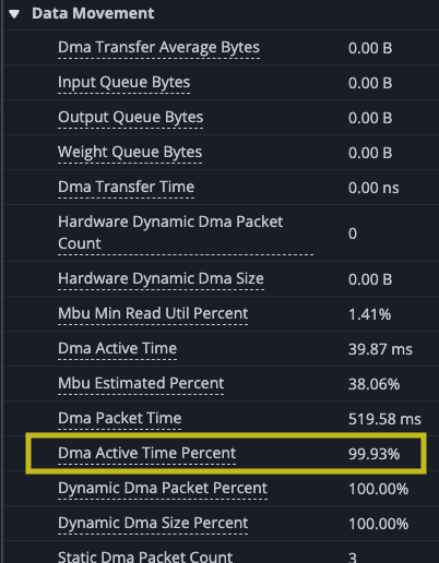
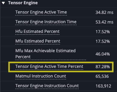
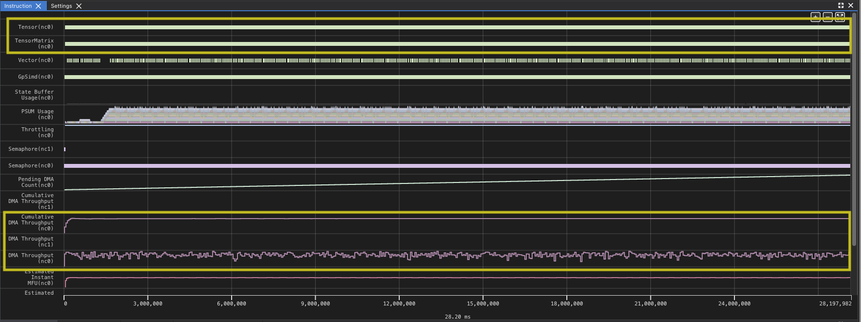
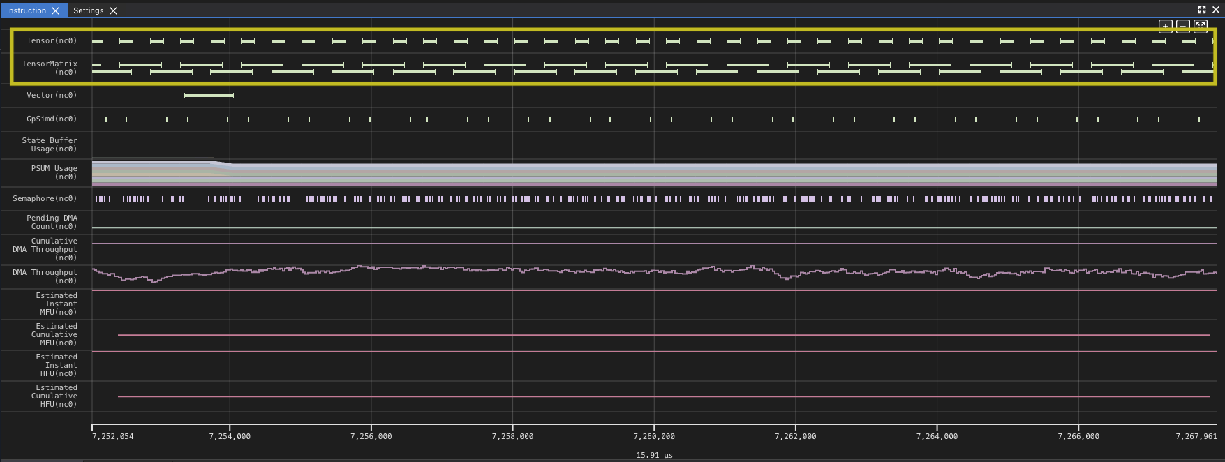
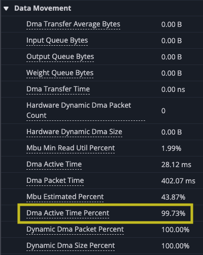
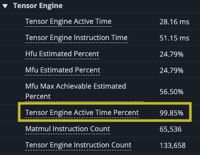
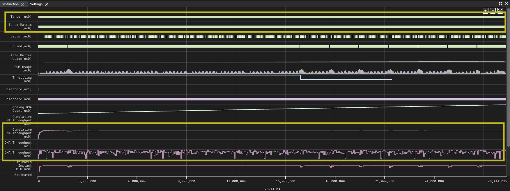
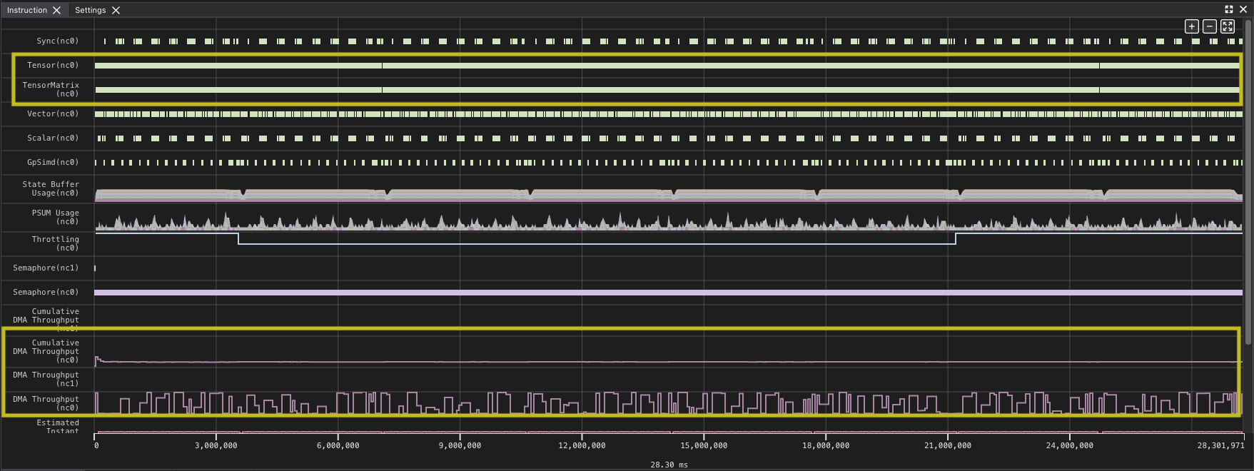
Looking at this profile for the full kernel run, you can see that the DMA queues which move data from HBM to SBUF and back are quite active. Looking at the Tensor and TensorMatrix lines, it appears there are some gaps within the run as well. The heavy use of DMA and the Tensor Engine (TensorE) is not too surprising, since those are the two things the kernel is primarily doing. The profile also provides some data as an overview of how much each engine is being used. You can zoom in to one of the areas where you see a gap and validate the impression.
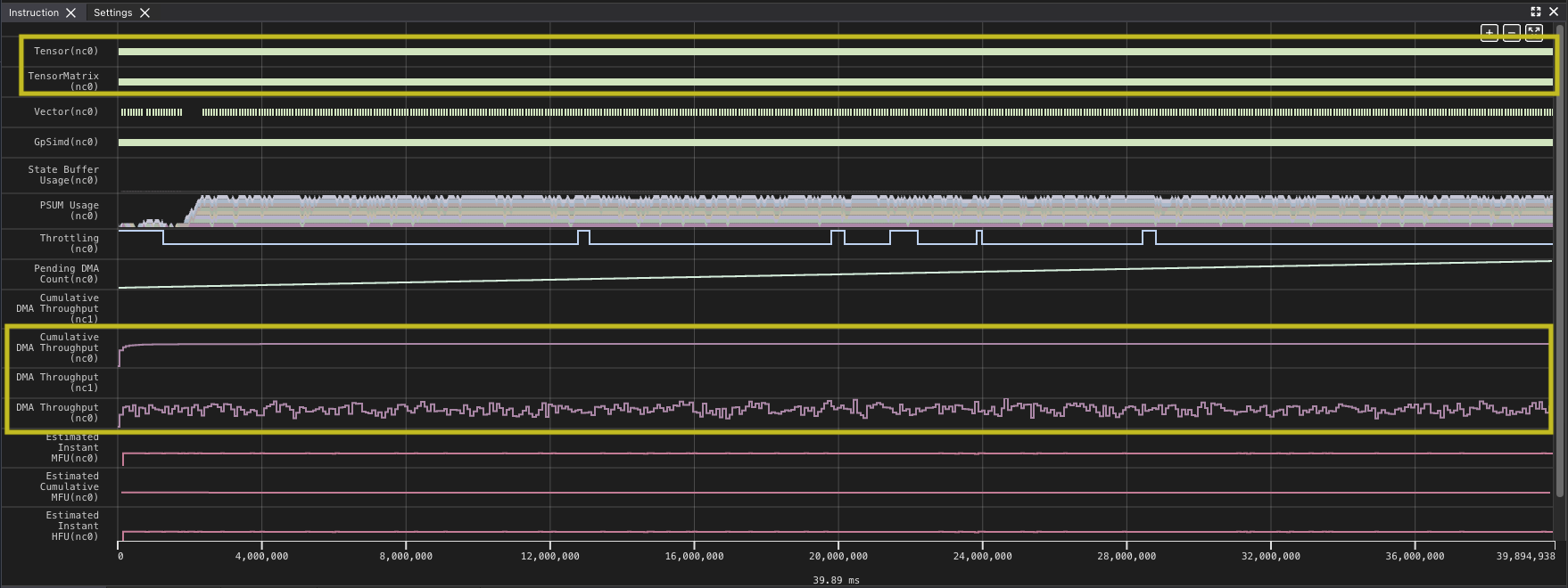
You can see that the TensorE is busy from the start of the kernel through the end. Note that matrix multiply becomes two instructions on the hardware load weights, which loads the static matrix, and matrix multiply, which loads the moving matrix and performs the matrix multiply operation.
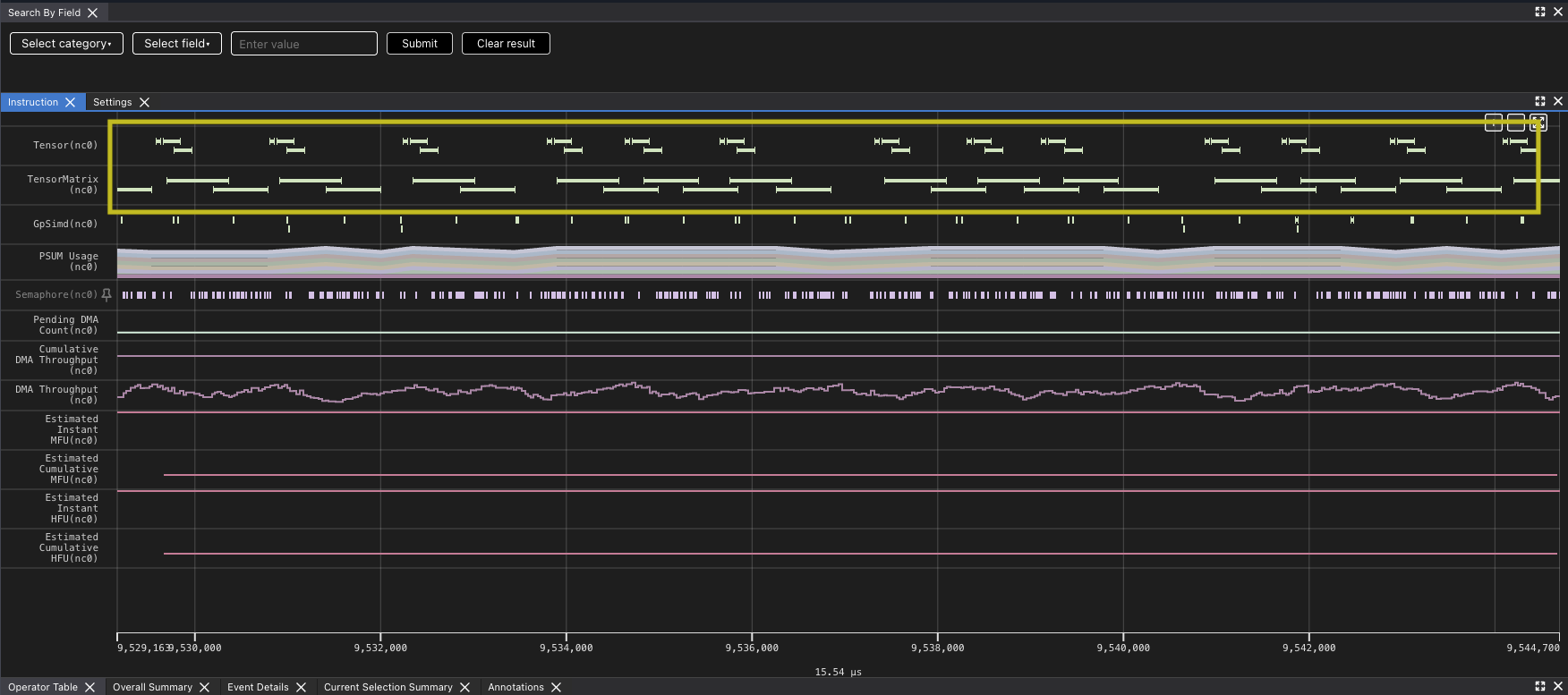
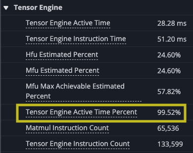
However, there are gaps between matrix multiply operations indicate that the TensorE is waiting on data to be read from the HBM to SBUF for the next operation to take place that we can see when we zoom in.Looking at the original kernel code you can see that you are loading the two tiles before each matrix multiply. Looking at the summary data provided in the profile, you can also see that the DMA engines were active 99.93% of the time while the TensorE was only active 87.28% of the run.
|
|
Analyzing the kernel#
The first step to improving the performance of the kernel is to analyze the performance you observed and apply that to your understanding of the NeuronEngine Architecture. The NeuronEngine Architecture consists of a number of computational engines that can each run independently, assuming the inputs are available for each instruction. In the current example, the only computational engine you are using is the TensorE and all of its inputs are coming directly from the DMA engines just before the computation is performed with the output of each tile written back after the k inner-most loop completes. Considering that matrix multiply is compute bound, you would expect that the matrix multiply instruction should be the limiting factor of your performance. However, TensorE was only active about 69.83% of the time, which tells us you can likely get more data to it faster to improve the overall computation time.
Looking at this, you might notice two things. First, since the data for each matrix multiply is being loaded just before the multiply, you are always waiting on these loads to complete before you can start the next multiply. If you look at the structure of the iteration, you can also see that you will load the same tile more than once. For instance the m=0, k=0 tile will be loaded N // TILE_N times. One change you could make is to load all of the tiles needed to compute a given output tile before you start the computation. You can accomplish this by moving the loads out into the outer loops, loading all K // TILE_K tiles for a given value of m from the stationary matrix at the start of the m loop, and all K // TILE_K tiles for a given value of n from the stationary matrix at the start of the n loop.
import nki
import nki.language as nl
import nki.isa as nisa

@nki.jit(platform_target="trn2")
def matrix_multiply_kernel(lhsT, rhs):
  """NKI kernel to compute a matrix multiplication operation in a tiled manner
     while hoisting the load of the lhsT and rhs to outer loops.

  Args:
      lhsT: an input tensor of shape [K,M], where both K and M are multiples for
        128.  It is the left-hand-side argument of the matrix multiplication,
        delivered transposed for optimal performance.
      rhs: an input tensor of shape [K,N], where K is a multiple of 128, and N
        is a multiple of 512.  It is the right-hand-side argument of the matrix
        multiplication.
  Returns:
      result: the resulting output tensor of shape [M,N]
  """

  # Verify that the lhsT and rhs are the expected sizes.
  K, M = lhsT.shape
  K_, N = rhs.shape
  assert K == K_, "lhsT and rhs must have the same contraction dimension"
  result = nl.ndarray(shape=(M, N), dtype=nl.float32, buffer=nl.hbm)

  # Lookup the device matrix multiply dimensions.
  TILE_M = nl.tile_size.gemm_stationary_fmax  # 128
  TILE_K = nl.tile_size.pmax  # 128
  TILE_N = nl.tile_size.gemm_moving_fmax  # 512

  # Verify that the input matrices are a multiple of the tile dimensions.
  assert M % TILE_M == 0, \
    f"Expected M, {M}, to be a multiple of stationary free-dimension max, {TILE_M}"
  assert N % TILE_N == 0, \
    f"Expected N, {N}, to be a multiple of moving free-dimension max, {TILE_N}"
  assert K % TILE_K == 0, \
    f"Expected K, {K}, to be a multiple of the partition dimension max, {TILE_K}"

  # Use affine_range to loop over tiles
  for m in nl.affine_range(M // TILE_M):
    # Load a whole column tiles from lhsT (with K * TILE_M numbers)
    # This corresponds to the whole row in the original lhs
    lhsT_tiles = []
    for k in nl.affine_range(K // TILE_K):
      # Allocate space in SBUF for the tile (uninitialized)
      lhsT_tile = nl.ndarray(shape=(TILE_K, TILE_M),
                           dtype=lhsT.dtype,
                           buffer=nl.sbuf)
      # Copy the tile from HBM to SBUF
      nisa.dma_copy(dst=lhsT_tile,
                  src=lhsT[k * TILE_K:(k + 1) * TILE_K,
                         m * TILE_M:(m + 1) * TILE_M])
      # Append the tile to the list of tiles.
      lhsT_tiles.append(lhsT_tile)

    for n in nl.affine_range(N // TILE_N):
      # Load a whole column tiles from rhs (with K * TILE_N numbers)
      rhs_tiles = []
      for k in nl.affine_range(K // TILE_K):
        # Allocate space in SBUF for the tile (uninitialized)
        rhs_tile = nl.ndarray(shape=(TILE_K, TILE_N),
                          dtype=rhs.dtype,
                          buffer=nl.sbuf)
        # Copy the tile from HBM to SBUF
        nisa.dma_copy(dst=rhs_tile,
                  src=rhs[k * TILE_K:(k + 1) * TILE_K,
                          n * TILE_N:(n + 1) * TILE_N])
        # Append the tile to the list of tiles.
        rhs_tiles.append(rhs_tile)

      # Allocate a tile in PSUM for the result
      result_tile = nl.ndarray(shape=(TILE_M, TILE_N),
                           dtype=nl.float32,
                           buffer=nl.psum)
      for k in nl.affine_range(K // TILE_K):
        # Accumulate partial-sums into PSUM
        nisa.nc_matmul(dst=result_tile,
                   stationary=lhsT_tiles[k],
                   moving=rhs_tiles[k])

      # Copy the result from PSUM back to SBUF, and cast to expected
      # output data-type
      result_tmp = nl.ndarray(shape=(TILE_M, TILE_N),
                          dtype=nl.float32,
                          buffer=nl.sbuf)
      nisa.tensor_copy(dst=result_tmp, src=result_tile)

      # Copy the result from SBUF to HBM.
      nisa.dma_copy(dst=result[m * TILE_M:(m + 1) * TILE_M,
                           n * TILE_N:(n + 1) * TILE_N],
                src=result_tmp)

  return result
The test program validates that the new implementation is correct and also provides new NEFF and NTFF.
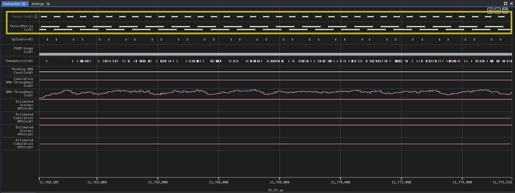
At this level the profile does not look too different, however when you zoom in, you can see that the matrix multiplies no longer show so many gaps.
Analyzing the improvement though, you can see that this change has made big strides. The DMA and matrix multiply is better overlapped, the DMA engines are now busy 99.73% of the time, slightly more than before, but the TensorE is busy 99.85% of the time. This is a huge improvement, but the time spent in the kernel is still dominated by DMA.
|
|
Overlapping data and compute through blocking#
The previous refinement of the kernel showed that you can improve the utilization of the TensorE by improving how the data is loaded. Instead of loading each tile in the innermost loop, lifting the loads to the outer loops and loading a whole column from both the transposed stationary matrix and the moving matrix reduced the overall amount data that needed to be moved from HBM to SBUF. However, the fact that the kernel is still memory bound means there is more that can be done.
Blocking is a technique to help load even larger amounts of data in at a time. Instead of copying single tiles of data from HBM to SBUF, you can load a full block, which is a multiple of the number of tiles. Since matrix multiply still needs to operate tile by tile, you compute all of the tiles in the block before proceeding to the next block.
import nki
import nki.language as nl
import nki.isa as nisa

@nki.jit(platform_target="trn2")
def matrix_multiply_kernel(lhsT, rhs):
  """NKI kernel to compute a matrix multiplication operation while blocking the
     free dimensions of the LHS and RHS to improve memory access pattern.

  Args:
      lhsT: an input tensor of shape [K,M], where both K and M are multiples for
        1.    It is the left-hand-side argument of the matrix multiplication,
        delivered transposed for optimal performance.
      rhs: an input tensor of shape [K,N], where K is a multiple of 128, and N
        is a multiple of 512.  It is the right-hand-side argument of the matrix
        multiplication.
  Returns:
      result: the resulting output tensor of shape [M,N]
  """

  # Verify that the lhsT and rhs have the same contraction dimension.
  K, M = lhsT.shape
  K_, N = rhs.shape
  assert K == K_, "lhsT and rhs must have the same contraction dimension"

  # Lookup the device matrix multiply dimensions.
  TILE_M = nl.tile_size.gemm_stationary_fmax  # 128
  TILE_K = nl.tile_size.pmax  # 128
  TILE_N = nl.tile_size.gemm_moving_fmax  # 512

  # Configuring the blocking size for the free dimensions
  TILES_IN_BLOCK_M = 2
  TILES_IN_BLOCK_N = 2

  BLOCK_M = TILE_M * TILES_IN_BLOCK_M  # 256
  BLOCK_N = TILE_N * TILES_IN_BLOCK_N  # 1024

  # the size has to be multiple of block size
  assert M % BLOCK_M == 0, f"Expected M ({M}) to be divisible by BLOCK_M ({BLOCK_M})"
  assert N % BLOCK_N == 0, f"Expected N ({N}) to be divisible by BLOCK_N ({BLOCK_N})"

  # Create a space for the result in HBM (not initialized)
  result = nl.ndarray(shape=(M, N), dtype=lhsT.dtype, buffer=nl.hbm)

  # Loop over blocks over the M dimension
  for m in nl.affine_range(M // BLOCK_M):
    # Load TILES_IN_BLOCK_M columns tiles from lhsT
    lhsT_tiles = []
    for bm in nl.affine_range(TILES_IN_BLOCK_M):
      # Inner tile array.
      lhsT_tiles_internal = []
      for k in nl.affine_range(K // TILE_K):
        # Allocate space in SBUF for the tile (uninitialized)
        lhsT_tile = nl.ndarray(shape=(TILE_K, TILE_M),
                               dtype=lhsT.dtype,
                               buffer=nl.sbuf)
        # Copy the tile from HBM to SBUF
        nisa.dma_copy(dst=lhsT_tile,
                src=lhsT[k * TILE_K:(k + 1) * TILE_K,
                     (m * TILES_IN_BLOCK_M + bm) *
                     TILE_M:((m * TILES_IN_BLOCK_M + bm) + 1) *
                     TILE_M])
        # Append the tile to the inner list of tiles.
        lhsT_tiles_internal.append(lhsT_tile)
      # Append the inner list of tiles into the outer list of tiles.
      lhsT_tiles.append(lhsT_tiles_internal)

    for n in nl.affine_range(N // BLOCK_N):
      # Load TILES_IN_BLOCK_N columns from rhs
      rhs_tiles = []
      for bn in nl.affine_range(TILES_IN_BLOCK_N):
        # Inner tile array.
        rhs_tiles_internal = []
        for k in nl.affine_range(K // TILE_K):
          # Allocate space in SBUF for the tile (uninitialized)
          rhs_tile = nl.ndarray(shape=(TILE_K, TILE_N),
                                dtype=rhs.dtype,
                                buffer=nl.sbuf)
          # Copy the tile from HBM to SBUF
          nisa.dma_copy(dst=rhs_tile,
                src=rhs[k * TILE_K:(k + 1) * TILE_K,
                    (n * TILES_IN_BLOCK_N + bn) *
                    TILE_N:((n * TILES_IN_BLOCK_N + bn) + 1) *
                    TILE_N])
          # Append the tile to the inner list of tiles.
          rhs_tiles_internal.append(rhs_tile)
        # Append the inner list of tiles into the outer list of tiles.
        rhs_tiles.append(rhs_tiles_internal)

      for bm in nl.affine_range(TILES_IN_BLOCK_M):
        for bn in nl.affine_range(TILES_IN_BLOCK_N):
          # Allocate a tensor in PSUM
          result_tile = nl.ndarray(shape=(TILE_M, TILE_N),
                                   dtype=nl.float32,
                                   buffer=nl.psum)
          for k in nl.affine_range(K // TILE_K):
            # Accumulate partial-sums into PSUM
            nisa.nc_matmul(dst=result_tile,
                           stationary=lhsT_tiles[bm][k],
                           moving=rhs_tiles[bn][k])

          # Copy the result from PSUM back to SBUF, and cast to expected
          # output data-type
          result_tmp = nl.ndarray(shape=result_tile.shape,
                                  dtype=result.dtype,
                                  buffer=nl.sbuf)
          nisa.tensor_copy(dst=result_tmp, src=result_tile)

          # Copy the result from SBUF to HBM.
          nisa.dma_copy(dst=result[(m * TILES_IN_BLOCK_M + bm) *
                                   TILE_M:((m * TILES_IN_BLOCK_M + bm) + 1) *
                                   TILE_M,
                                   (n * TILES_IN_BLOCK_N + bn) *
                                   TILE_N:((n * TILES_IN_BLOCK_N + bn) + 1) *
                                   TILE_N],
                        src=result_tmp)

  return result
Running the test driver ensures the new implementation of the kernel is correct and provides a new NEFF and NTFF that helps us understand the improvements.
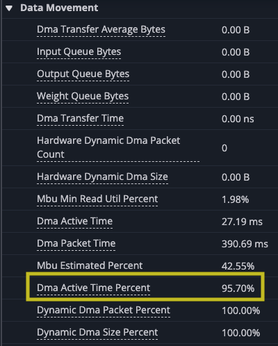
Zooming in on a similarly sized section shows that while the overall time of the kernel has improved, there are again gaps between our matrix multiply instructions.
Again you can see gaps in the matrix multiply. Even though the new implementation of the kernel improves on the overall time of the kernel, the new implementation reduces the number of DMA instructions, because each instruction loads more, but you wait longer for each block to load. In fact, even though the performance improved the TensorE is actually less utilized as a percentage of time, dropping to 99.52% of the time, with the DMA engines hitting 95.70%. This means there is a small amount of time when only the TensorE is being used, but the DMA engine is still active for most of the kernel run, which you should expect could be smaller.
|
|
Optimizing DMA through blocking the contraction dimension#
One of the advantages of leaving the K dimension unblocked was that you could rely on the PSUM buffer to hold the final computed value. To block in the K dimension, you will need to store intermediate partial sums in a temporary SBUF array of tiles. The nki.isa.tensor_tensor instruction can be used to add two tensors, allowing you to accumulate into the temporary tile. With this, you can build blocks in all three dimensions. This version of blocking loads the blocks to in BLOCK_K by BLOCK_M and BLOCK_K by BLOCK_N dimensions.
import nki
import nki.language as nl
import nki.isa as nisa


@nki.jit(platform_target="trn2")
def matrix_multiply_kernel(
    lhsT,
    rhs,
    # Meta-parameters
    TILES_IN_BLOCK_M=16,
    TILES_IN_BLOCK_N=2,
    TILES_IN_BLOCK_K=8,
):
  """NKI kernel to compute a large matrix multiplication efficiently by
     blocking all dimensions and doing layout optimization.

  Args:
      lhsT: an input tensor of shape [K,M], where K is a multiple of 128 *
        TILES_IN_BLOCK_K and M is a multiple of 128 * TILES_IN_BLOCK_M.  It is the
        left-hand-side argument of the matrix multiplication, delivered transposed
        for optimal performance.
      rhs: an input tensor of shape [K,N],  where K is a multiple of 128 *
        TILES_IN_BLOCK_K and N is a multiple of 512 * TILES_IN_BLOCK_N.  It is
        the right-hand-side argument of the matrix multiplication.
      TILES_IN_BLOCK_*: meta parameters to control blocking dimensions
  Returns:
      result: the resulting output tensor of shape [M,N]
  """

  # Verify that the lhsT and rhs have the same contraction dimension.
  K, M = lhsT.shape
  K_, N = rhs.shape
  assert K == K_, "lhsT and rhs must have the same contraction dimension"

  # Lookup the device matrix multiply dimensions.
  TILE_M = nl.tile_size.gemm_stationary_fmax  # 128
  TILE_K = nl.tile_size.pmax  # 128
  TILE_N = nl.tile_size.gemm_moving_fmax  # 512

  # Compute the block dimensions.
  BLOCK_M = TILE_M * TILES_IN_BLOCK_M
  BLOCK_N = TILE_N * TILES_IN_BLOCK_N
  BLOCK_K = TILE_K * TILES_IN_BLOCK_K

  # the size has to be multiple of block size
  assert M % BLOCK_M == 0, \
    f"Expected M {M} to be divisble by {BLOCK_M} when there are {TILES_IN_BLOCK_M}"
  assert N % BLOCK_N == 0, \
    f"Expected N {N} to be divisble by {BLOCK_N} when there are {TILES_IN_BLOCK_N}"
  assert K % BLOCK_K == 0, \
    f"Expected K {K} to be divisble by {BLOCK_K} when there are {TILES_IN_BLOCK_K}"

  # Create a space for the result in HBM (not initialized)
  result = nl.ndarray(shape=(M,N), dtype=nl.float32, buffer=nl.hbm)

  # Compute the number of blocks in each dimension
  NUM_BLOCK_M = M // BLOCK_M
  NUM_BLOCK_N = N // BLOCK_N
  NUM_BLOCK_K = K // BLOCK_K

  # Blocking N dimension (the RHS free dimension)
  for n in nl.affine_range(NUM_BLOCK_N):
    # Create the initial result tiles in SBUF and initialize each tile to
    # 0.0, since the final results will be accumulated here.
    result_tmps = []
    for m_idx in range(NUM_BLOCK_M):
      block_m = []
      for bm_idx in range(TILES_IN_BLOCK_M):
        block_n = []
        for bn_idx in range(TILES_IN_BLOCK_N):
          # Create the result tile (uninitialized)
          tile = nl.ndarray(shape=(TILE_M, TILE_N),
                            dtype=lhsT.dtype,
                            buffer=nl.sbuf)
          # Initialize the tile 0.0
          nisa.memset(dst=tile, value=0.0)
          # Append the tile to block_n array.
          block_n.append(tile)
        # Append block_n array to block_m array.
        block_m.append(block_n)
      # Append block_m array into result_tmps.
      result_tmps.append(block_m)

    # Blocking K dimension (the contraction dimension)
    # Use `sequential_range` because we do not want the compiler to
    # change this loop by, for example, vectorizing it
    for k in nl.sequential_range(NUM_BLOCK_K):
      # Loading tiles from rhs setting the load tile to
      # `TILE_K x BLOCK_SIZE_N` to optimize DMA performance
      rhs_tiles = []
      for bk_r in range(TILES_IN_BLOCK_K):
        # Allocate rhs_tile tensor, TILE_K x BLOCK_N
        rhs_tile = nl.ndarray(shape=(TILE_K, BLOCK_N),
                              dtype=rhs.dtype,
                              buffer=nl.sbuf)
        # Copy block tile from rhs, to rhs_tile.
        nisa.dma_copy(dst=rhs_tile[0:TILE_K, 0:BLOCK_N],
                      src=rhs[(TILES_IN_BLOCK_K * k + bk_r) *
                              TILE_K:(TILES_IN_BLOCK_K * k + bk_r + 1) * TILE_K,
                              BLOCK_N * n:BLOCK_N * (n + 1)])
        # Append rhs_tile to rhs_tiles.
        rhs_tiles.append(rhs_tile)

      # Blocking M dimension (the LHS free dimension)
      for m in nl.affine_range(NUM_BLOCK_M):
        # Loading tiles from lhsT
        lhsT_tiles = []
        for bk_l in nl.affine_range(TILES_IN_BLOCK_K):
          # Allocate lhsT_tile in SBUF (uninitialized)
          lhsT_tile = nl.ndarray(shape=(TILE_K, BLOCK_M),
                                 dtype=lhsT.dtype,
                                 buffer=nl.sbuf)
          # Copy block tile from lhsT to lhsT_tile
          nisa.dma_copy(
            dst=lhsT_tile[0:TILE_K, 0:BLOCK_M],
            src=lhsT[(TILES_IN_BLOCK_K * k + bk_l) *
                 TILE_K:(TILES_IN_BLOCK_K * k + bk_l + 1) * TILE_K,
                 BLOCK_M * m:BLOCK_M * (m + 1)])
          # Copy block tile from lhsT to lhsT_tile
          lhsT_tiles.append(lhsT_tile)

        # Do matmul with all tiles in the blocks
        for bn in nl.affine_range(TILES_IN_BLOCK_N):
          for bm in nl.affine_range(TILES_IN_BLOCK_M):
            # Allocate result_tile in PSUM (uninitialized)
            result_tile = nl.ndarray(shape=(TILE_M, TILE_N),
                                     dtype=nl.float32,
                                     buffer=nl.psum)
            for bk in nl.affine_range(TILES_IN_BLOCK_K):
              # Perform matrix multiply on a tile.
              nisa.nc_matmul(
                dst=result_tile,
                stationary=lhsT_tiles[bk][0:TILE_K, bm * TILE_M:(bm + 1) * TILE_M],
                moving=rhs_tiles[bk][0:TILE_K, bn * TILE_N:(bn + 1) * TILE_N]
              )
            # Accumulate the result into the result_tmps tile.
            nisa.tensor_tensor(dst=result_tmps[m][bm][bn],
                               data1=result_tmps[m][bm][bn],
                               data2=result_tile,
                               op=nl.add)

    # Copying the result from SBUF to HBM
    for m in nl.affine_range(NUM_BLOCK_M):
      for bm in nl.affine_range(TILES_IN_BLOCK_M):
        # coalesce result tiles for better DMA performance
        result_packed = nl.ndarray(shape=(TILE_M, BLOCK_N),
                                   dtype=nl.float32,
                                   buffer=nl.sbuf)
        for bn in nl.affine_range(TILES_IN_BLOCK_N):
          nisa.tensor_copy(
            dst=result_packed[0:TILE_M, bn * TILE_N:(bn + 1) * TILE_N],
            src=result_tmps[m][bm][bn][0:TILE_M, 0:TILE_N])

        # Copy packed result from SBUF to HBM.
        nisa.dma_copy(dst=result[(TILES_IN_BLOCK_M * m + bm) *
                                 TILE_M:(TILES_IN_BLOCK_M * m + bm + 1) * TILE_M,
                                 BLOCK_N * n:BLOCK_N * (n + 1)],
                      src=result_packed[0:TILE_M, 0:BLOCK_N])

  return result
This version of the kernel is considerably more complicated, but the test driver you created for the simplest version of this kernel means you have a ready test. The sizes of matrices you chose in the original test were forward-looking in that they correspond to the tiling dimensions you selected. However, you expose these as additional arguments (unlike in the previous blocking), so a model calling this kernel can choose block sizes appropriate for the model. The test driver also gives us a new set of NEFF and NTFF files.
Other than the improved time, this seems similar to the other profile graphs, however you can see a slightly more complex pattern. This reflects the time to compute the full output tile and then copying the results out.
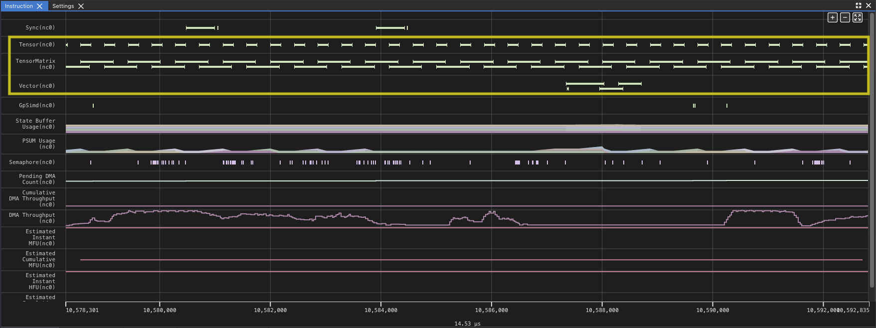
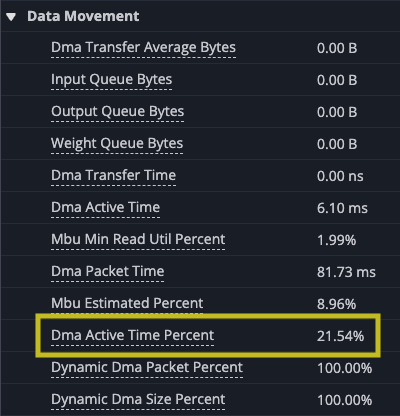
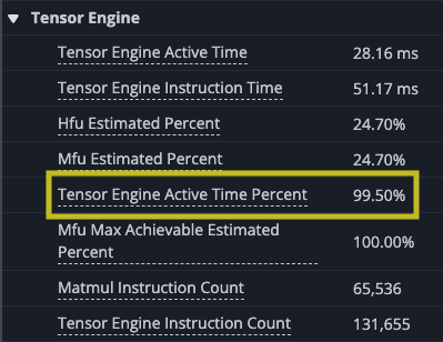
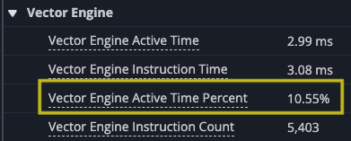
Zooming in you can see the gap at the end of the set of matrix multiplies where the results are accumulated into the SBUF temporary results. Looking at the utilization of the DMA engines and TensorE you can see the DMA engines are now active only 21.54% of the time, while the TensorE is now active 99.50%, with the Vector Engine (VectorE) active 10.55% of the time, where it was previously unused.
|
|
|
This final version of the matrix multiply kernel is no longer memory-bound. Instead, as you should expect, it is compute-bound with the TensorE and VectorE engines being the limiting factor on the speed of the kernel.
Summary#
While the matrix multiply example kernel is a relatively simple one, which primarily focuses on just two of the engines in the NeuronEngine Architecture: the DMA engines and the TensorE, it demonstrates how you can start with a simpler known correct version of a kernel with a test case that provides a representative workload and use a combination of your understanding of the NeuronEngine Architecture, the Neuron Profiler, and your understanding of the kernel you are trying to implement to improve the performance of the kernel.
Once the kernel is ready you use it to replace the section of the model it is intended to implement. The test driver can continue to be used as a unit test that ensures correct operations and allows you to add regression tests, both for accuracy and performance of the kernel. It can also provide a starting point to porting to other generations of the NeuronEngine Architecture.