Introduction to Direct Memory Access (DMA) with NKI

Direct Memory Access (DMA) engines in Neuron enable efficient data movement between different memory types, primarily between the device memory (HBM) and on-chip SRAM buffers (SBUF). DMA Engines can operate in parallel to compute, allowing asynchronous data movement independent from compute operations. Each NeuronCore (v2-v4) is paired with 16 DMA engines. Understanding and efficiently utilizing these DMA engines is critical for maximizing memory bandwidth utilization and overall workload performance.

Before reading this doc, it may be helpful to refer to Introduction to memory hierarchy in NKI.

Basic DMA Capabilities

To move data between HBM and SBUF, programmers can initiate a DMA transfer that gets executed by the DMA engines. Each DMA transfer starts with a DMA trigger from a NeuronCore and ends with a semaphore update from the DMA engine to signal the completion of transfer back to the NeuronCore. Today, each DMA transfer is by default parallelized up to 16 DMA engines, depending on the shape.

The 16 DMA Engines are connected to both the off chip HBM and the on-chip SRAM, called SBUF. DMA transfers can move data in multiple directions: bidirectionally between HBM to SBUF, within HBM or within SBUF. Each DMA engine has a theoretical bandwidth of 27.2 GB/s for NeuronCore-v2 and -v3 or 38.4 GB/s for NeuronCore-v4. DMA engines also support scatter-gather operations, allowing a single transfer to gather data from multiple non-contiguous source buffers or scatter to multiple non-contiguous destination buffers.

DMA transfers can perform both copy and transpose transfers into SBUF. This doc will mainly focus on copy transfers. You can also perform casting as part of DMA when the transfer has a different source and destination datatype. Neuron supported datatypes can be found in the NKI datatype guide. The casting operation is performed by first casting the source type to FP32, before finally casting to the destination type. This may be worth considering if working with integer types. Casting with DMAs is not supported for MXFP4 and MXFP8 datatypes.

DMA Triggers

DMA transfers can be triggered by any engine sequencer in the NeuronCore. (For details, refer to Trainium2 Architecture Guide for NKI.) The sequencer instruction to trigger the transfer may wait on any semaphore condition which is signaled by other compute engines to respect data dependencies. The engine associated to the sequencer triggering the associated DMA is referred to as the “Trigger Engine” for a given DMA Transfer. The Trigger Engine for a given transfer can be specified via the engine parameter in nisa.dma_copy.

DMA Queues

DMA transfers are submitted to DMA queues for the DMA Engines to consume. There are 16 DMA queues per DMA engine (ID 0-15). A given DMA transfer can be submitted to a single queue ID across all 16x DMA engines paired with a NeuronCore. The given queue for a DMA transfer can be seen when mousing over a DMA transfer in a profile in Neuron Explorer. The queue ID is typically tied to the trigger engine and the method of descriptor generation (refer to the NeuronCore-v3 architecture guide for details). DMA transfers within a queue on the same DMA engine are executed in order. DMA transfers from different DMA queues are scheduled in a round robin fashion (for NeuronCore-v2 and v3) or based on the queue QoS configured (for NeuronCore-v4). Refer to the NeuronCore-v4 architecture guide for more details on DMA QoS.

Performance Considerations

When moving data in or out of SBUF, optimal performance is achieved with transfers maximizing the number of partitions with 4KiB or larger per partition. Given 16x DMA engines and 128 SBUF partitions, each DMA engine is typically responsible for moving data for eight SBUF partitions (128 partitions / 16 DMA engines). The figure below visualizes the DMA throughput across different number of bytes per partition (“Free Bytes”), for a fixed partition dimension size of 128:

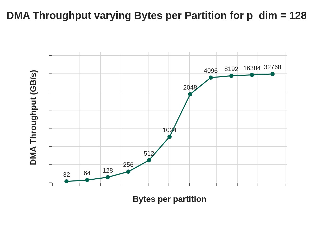
The points on the graph refer to various Free (Dimension) Byte values (that is, bytes per partition). We see that at 4096 free bytes, we are able to nearly saturate DMA bandwidth. In the DMA Deep Dive, we will review a techniques for reshaping/folding input tensors to increasing free dimension read sizes.

Another key consideration for performance is overhead to initiate a DMA transfer. Small, frequent transfers incur significant overhead causing us to be latency bound, while larger transfers help amortize these costs, moving to a more bandwidth bound regime. For optimal performance, it’s important to batch data movements into larger transfers whenever possible.

We will look at two examples below, which show various shapes, sizes and access patterns, and how this affects the the achieved DMA throughput of the corresponding DMA transfers.

Examples

As DMAs are a result of the corresponding source layout and access pattern, it is best to look at concrete examples to ground our understanding of common applications and their resulting access patterns.

Example 1: Move A[4,4096] HBM → SBUF

The purpose of this example is to show a very simple access pattern (a 2D tensor in contiguous memory in HBM, being written to SBUF). This should build a foundation of how a particular access pattern maps to a specific set of DMA transfers.

Consider a 2D Tensor, A[4, 4096], in HBM. Assume the tensor is laid out in row-major form and is contiguous in the HBM. In row major form, array elements are stored sequentially row by row in memory, meaning all elements of the first row are stored first, followed by all elements of the second row, and so on. Let’s assume we wish to move this tensor to SBUF, where the destination tensor will have a partition dimension of 4 and a free dimension of 4096. Each row of the source tensor will occupy a single partition in SBUF.

Assuming A is a bfloat16 tensor, this means that the total size of the tensor is 32KiB (4*4096*2B). Knowing that each DMA engine corresponds to 8 partition lanes, and we are writing our 4 rows to only 4 partition lanes of SBUF, we would expect to see a single DMA engine active, with a single transfer size of 32KiB.

Here is a diagram with the expected behavior:

Example

Here is the kernel to perform the DMA transfer.

import nki.language as nl
import nki.isa as nisa
import nki
import os

os.environ["NEURON_FRAMEWORK_DEBUG"] = "1"
os.environ["NEURON_RT_ENABLE_DGE_NOTIFICATIONS"] = "1"

@nki.jit(platform_target="trn2", mode="torchxla")
def tensor_exp_kernel_isa(in_tensor):
  """NKI kernel to compute elementwise exponential of an input tensor
  Args:
       in_tensor: an input tensor of shape [4,4096]
  Returns:
       out_tensor: an output tensor of shape [4,4096]
  """
  out_tensor = hbm.view(dtype="bfloat16", shape=in_tensor.shape)
  sbuf_tensor =  sbuf.view(dtype="bfloat16", shape=in_tensor.shape)
  out_tile =  sbuf.view(dtype="bfloat16", shape=in_tensor.shape)

  # Load input data from HBM to on-chip memory
  nisa.dma_copy(src=in_tensor[0:4, 0:4096], dst=sbuf_tensor)

  # perform the computation:
  out_tile = nisa.activation(op=nl.exp, data=sbuf_tensor)

  # store the results back to HBM
  nisa.dma_copy(src=out_tile, dst=out_tensor[0:4, 0:4096])
  return out_tensor

if __name__ == "__main__":
  import torch
  from torch_xla.core import xla_model as xm
  device = xm.xla_device()
  shape = (4,4096) # Tensor shape : [4,4096]
  in_tensor = torch.ones(shape,  dtype=torch.bfloat16).to(device=device)
  out_tensor = tensor_exp_kernel_isa(in_tensor)
  print(out_tensor) # an implicit XLA barrier/mark-step

Profile

The above code runs on a single NeuronCore-v3, in a Trn2 instance. Here we can look at the profile, to validate the expected behavior. Refer to the Neuron Explorer user guide for guidance on how to generate a profile.

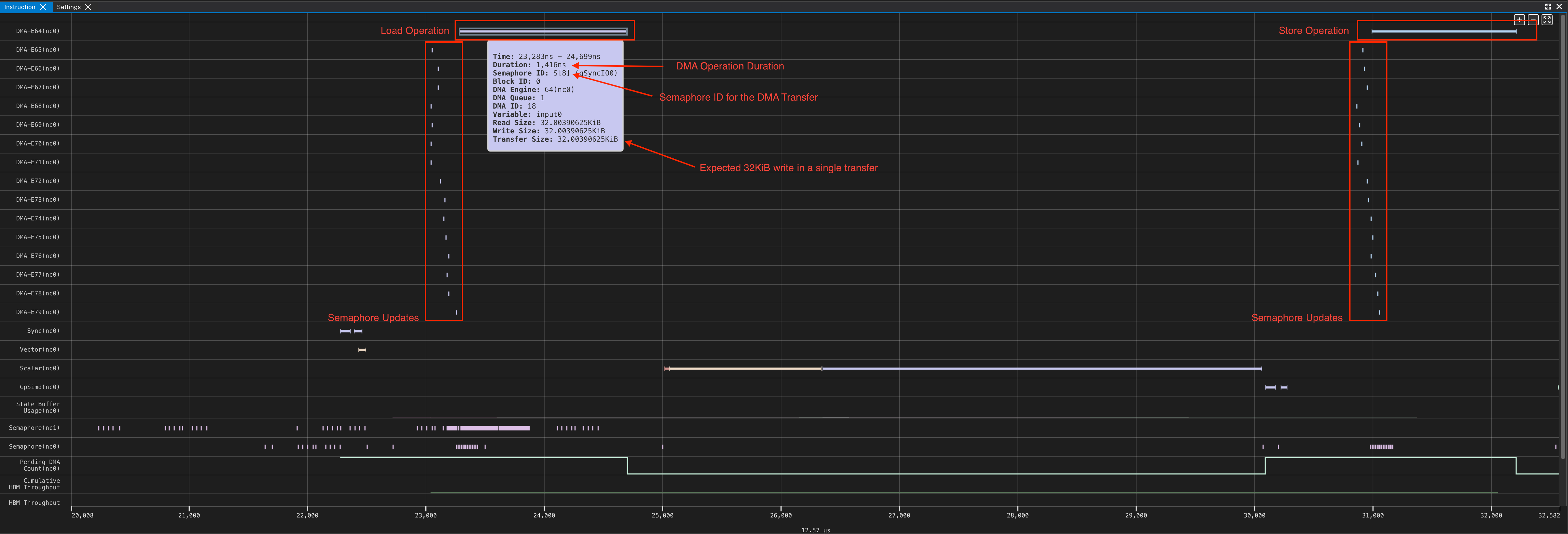
This is exactly what we expected based on our analysis. From the profile, we can see that the first DMA engine takes 1416 ns to load 32 KiB from HBM to SBUF and also a small 4B semaphore update. Even though the remaining 15 DMA engines do not perform useful data movement, they also perform a small 4B semaphore update writes. This allows the NeuronCore to always monitor a semaphore increment of 16 to signal DMA transfer completion, regardless of the tensor shapes in the transfer.

This is good, but this example only uses a single DMA engine. In the next example, we increase partition dimension to increase the number of DMA Engines in use.

Example 2: Move A[128,128] HBM → SBUF

The purpose of this example is to show how as partition count scales, the number of DMA Engines in use increases.

Consider a 2D Tensor A[128, 128] in HBM, laid out in row-major form and contiguous on the HBM. Assuming we wish to move A from HBM to SBUF, how many DMA engines will this require?

Again, we see the total tensor size is 32KiB (128*128*2B), the same as the previous example. We are writing across 128 partitions of SBUF, with each row corresponding to a partition lane. Knowing that each DMA engine corresponds to 8 partition lanes, and we are writing to 128 partitions, we would expect all 16 DMA engines to be active, each performing a single DMA operation of 2KiB (8 rows x 128 elements x 2 bytes per element).

Here is a diagram of the expected transfer:

Example

import nki.language as nl
import nki.isa as nisa
import nki
import os
os.environ["NEURON_FRAMEWORK_DEBUG"] = "1"
os.environ["NEURON_RT_ENABLE_DGE_NOTIFICATIONS"] = "1"


@nki.jit(platform_target="trn2", mode="torchxla")
def tensor_exp_kernel_isa(in_tensor):
  """NKI kernel to compute elementwise exponential of an input tensor
  Args:
        in_tensor: an input tensor of shape [128,128]
  Returns:
        out_tensor: an output tensor of shape [128,128]
  """
  out_tensor = hbm.view(dtype="bfloat16", shape=in_tensor.shape)
  sbuf_tensor =  sbuf.view(dtype="bfloat16", shape=in_tensor.shape)
  out_tile =  sbuf.view(dtype="bfloat16", shape=in_tensor.shape)

  # Load input data from HBM to on-chip memory
  nisa.dma_copy(src=in_tensor[0:128, 0:128], dst=sbuf_tensor)

  # perform the computation:
  out_tile = nisa.activation(op=nl.exp, data=sbuf_tensor)

  # store the results back to HBM
  nisa.dma_copy(src=out_tile, dst=out_tensor[0:128, 0:128])
  return out_tensor

if __name__ == "__main__":
  import torch
  import torch_xla


  device = torch_xla.device()
  shape = (128, 128) # Tensor shape : [128, 128]
  in_tensor = torch.ones(shape,  dtype=torch.bfloat16).to(device=device)
  print(in_tensor.dtype)
  out_tensor = tensor_exp_kernel_isa(in_tensor)
  print(out_tensor) # an implicit XLA barrier/mark-step

Profile

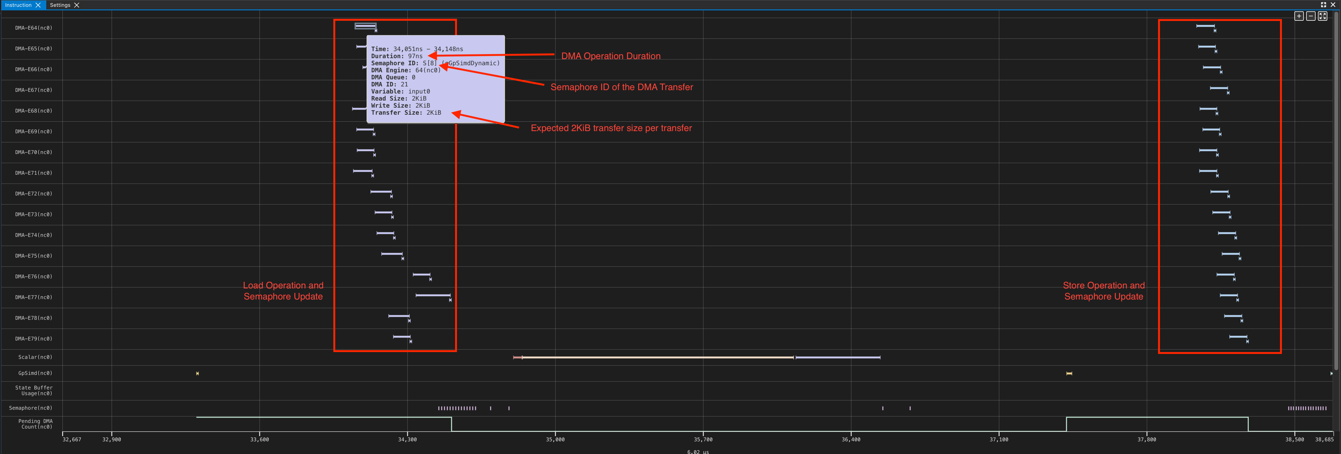
In the above profile, we can see that all 16 DMA engines are active, as each DMA engine is reading 8 rows from HBM and writing to 8 corresponding partition lanes in SBUF. Similarly, we see the reverse also applies from SBUF, back to HBM. By mousing over an individual DMA operation, we see each DMA engine corresponds to a single 2KiB read (8 rows x 128 elements x 2B), as we expect!

Using the same profile from the 128x128 DMA example, lets look at the DMA Trigger and the associated Transfer. You can trace the DMA trigger instruction and the associated DMA transfer via the profiler. This would be useful if you wanted to understand the why a DMA was triggered when, and any preceding dependencies.

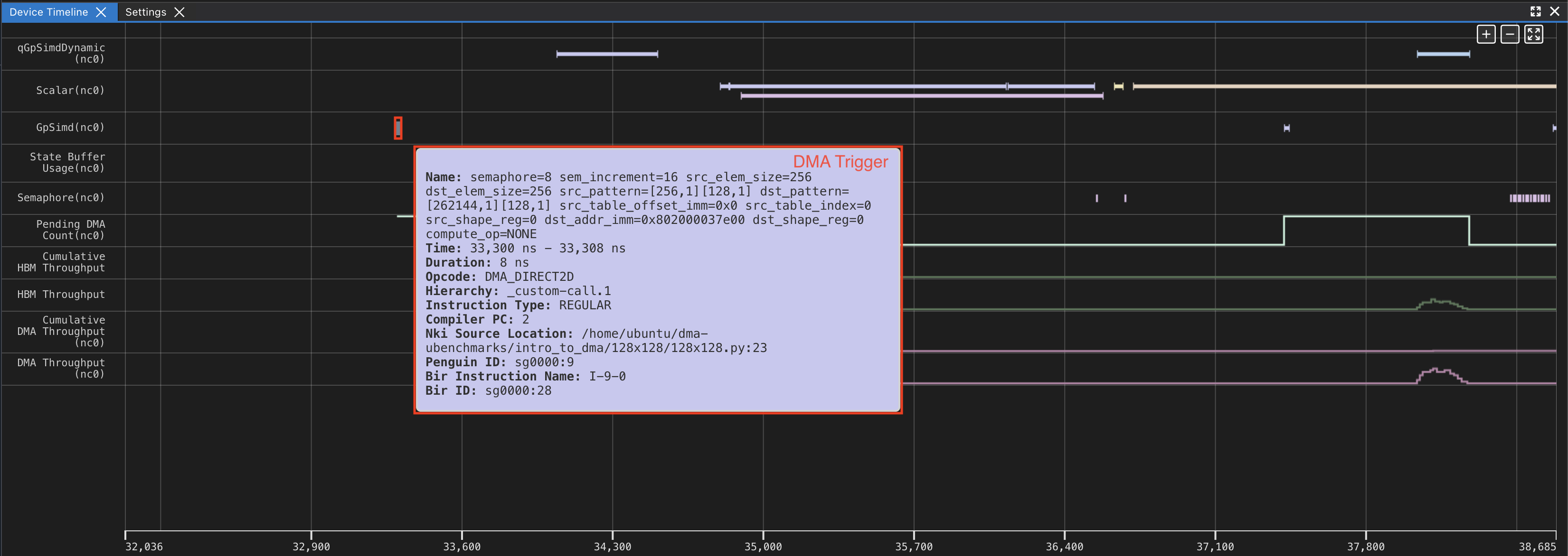
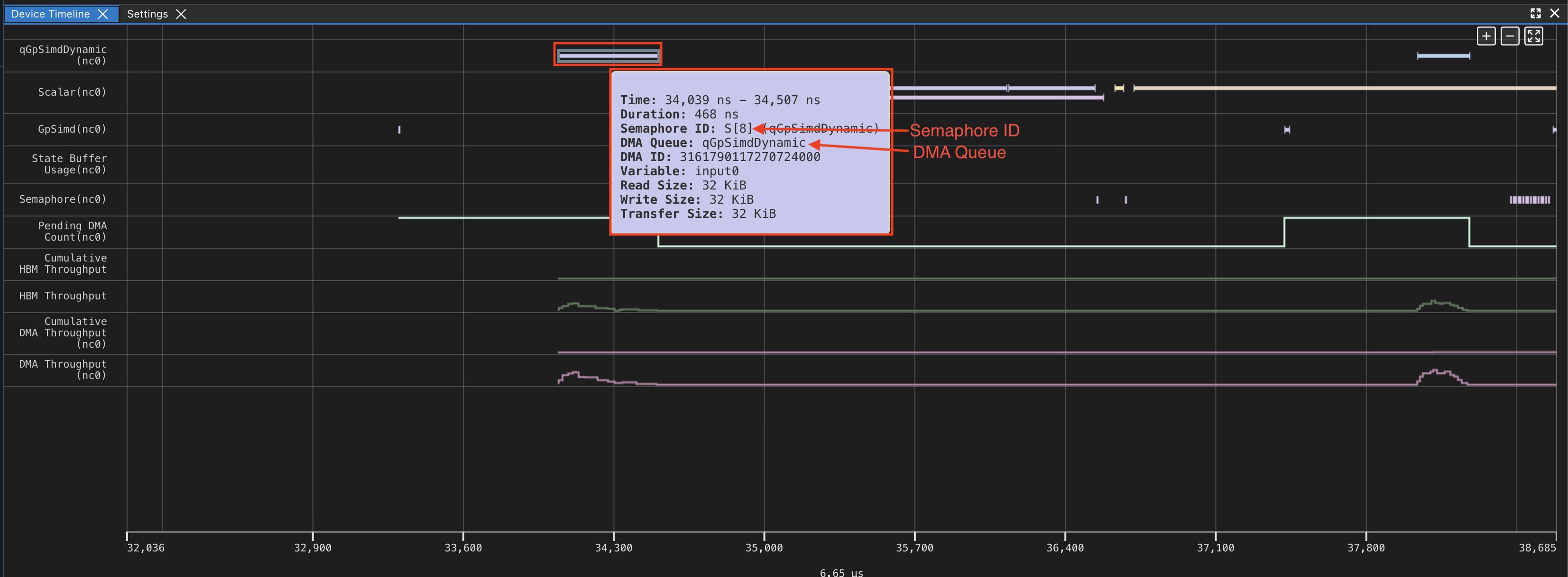
We can see the first DMA is triggered from qGpSimdDynamic (First screenshot). We can look at GPSimd to see the corresponding trigger (second screenshot).