How to Profile a NKI Kernel#
Learn how to profile Neuron Kernel Interface (NKI) kernels using Neuron Explorer to analyze hardware-level performance characteristics on Trainium and Inferentia devices. This comprehensive guide covers two profiling methods: using the neuron-profile capture command-line tool and the @nki.profile decorator API. You’ll discover how to generate NEFF and NTFF files, identify performance bottlenecks, optimize kernel execution, and leverage the interactive web-based Neuron Profile UI to visualize execution traces with source code integration for efficient NKI kernel development and optimization.
Install Neuron Explorer#
Ensure that you have the latest version of the aws-neuronx-tools package installed asNeuron Explorer comes with this package. The aws-neuronx-tools package is pre-installed on Neuron DLAMIs.
For detailed installation instructions, see: How to Get Started with Neuron Explorer.
Profile a NKI Kernel#
Profiling NKI (Neuron Kernel Interface) kernels helps you understand hardware level performance characteristics of your kernels running on AWS Trainium and Inferentia devices. When you write or optimize custom NKI kernels, profiling allows you to:
Identify bottlenecks: Determine if your kernel is compute-bound, memory-bound, or limited by data movement.
Optimize performance: Analyze kernel-level execution time, investigate compute engine utilization, look for opportunities to implement operator fusion to fine-tune performance.
Compare implementations: Benchmark different kernel implementations or configurations to pick the most efficient kernel.
You can profile NKI kernels using several approaches. In this guide, you’ll learn two primary methods for profiling NKI kernels.
Method #1: Profile using neuron-profile capture#
To profile an NKI kernel using neuron-profile capture, follow these three steps:
Set the environment variable
NEURON_FRAMEWORK_DEBUG=1to instruct the compiler to save the NEFF (Neuron Executable File Format) file.Execute the NKI kernel to generate the NEFF file.
Run
neuron-profile captureto create an Neuron Trace File Format (NTFF) file for performance analysis.
Each of these steps is explained in detail below.
Step 1: Set Environment Variables#
We will profile a 3-layer MLP model that fuses matrix multiplications with ReLU activation functions and uses a NKI matrix multiplication kernel. The rest of this tutorial will use a performance profile generated from this example. Here is the implementation of mlp_with_mm_kernel.py. Save this file before moving on to the next step:
"""
Example 3-layer MLP with matrix multiplication kernel to demonstrate Neuron Profile.
"""

import torch
import torch.nn as nn
import torch.nn.functional as F
import neuronxcc.nki as nki
import neuronxcc.nki.isa as nisa
import neuronxcc.nki.language as nl
import os

os.environ["NEURON_FRAMEWORK_DEBUG"] = "1"
os.environ["XLA_IR_DEBUG"] = "1"
os.environ["XLA_HLO_DEBUG"] = "1"


@nki.jit
def nki_matmul_fully_optimized_(
    lhsT,
    rhs,
    # Meta-parameters
    TILES_IN_BLOCK_M=16,
    TILES_IN_BLOCK_N=2,
    TILES_IN_BLOCK_K=8,
):
  """NKI kernel to compute a large matrix multiplication efficiently by
     blocking all dimensions and doing layout optimization.

  Args:
      lhsT: an input tensor of shape [K,M], where K is a multiple of 128 *
        TILES_IN_BLOCK_K and M is a multiple of 128 * TILES_IN_BLOCK_M.  It is the
        left-hand-side argument of the matrix multiplication, delivered transposed
        for optimal performance.
      rhs: an input tensor of shape [K,N],  where K is a multiple of 128 *
        TILES_IN_BLOCK_K and N is a multiple of 512 * TILES_IN_BLOCK_N.  It is
        the right-hand-side argument of the matrix multiplication.
      TILES_IN_BLOCK_*: meta parameters to control blocking dimensions
  Returns:
      result: the resulting output tensor of shape [M,N]
  """

  K, M = lhsT.shape
  K_, N = rhs.shape
  assert K == K_, "lhsT and rhs must have the same contraction dimension"
  result = nl.ndarray((M, N), dtype=lhsT.dtype, buffer=nl.shared_hbm)

  TILE_M = nl.tile_size.gemm_stationary_fmax  # 128
  TILE_K = nl.tile_size.pmax  # 128
  TILE_N = nl.tile_size.gemm_moving_fmax  # 512

  BLOCK_M = TILE_M * TILES_IN_BLOCK_M
  BLOCK_N = TILE_N * TILES_IN_BLOCK_N
  BLOCK_K = TILE_K * TILES_IN_BLOCK_K

  # the size has to be multiple of block size
  assert M % BLOCK_M == 0
  assert N % BLOCK_N == 0
  assert K % BLOCK_K == 0

  NUM_BLOCK_M = M // BLOCK_M
  NUM_BLOCK_N = N // BLOCK_N
  NUM_BLOCK_K = K // BLOCK_K

  # Blocking N dimension (the RHS free dimension)
  for n in nl.affine_range(NUM_BLOCK_N):
    result_tiles = nl.zeros((NUM_BLOCK_M, TILES_IN_BLOCK_M, TILES_IN_BLOCK_N,
                             nl.par_dim(TILE_M), TILE_N),
                            dtype=lhsT.dtype,
                            buffer=nl.sbuf)

    # Blocking K dimension (the contraction dimension)
    # Use `sequential_range` because we do not want the compiler to change this loop by,
    # for example, vectorizing it
    for k in nl.sequential_range(NUM_BLOCK_K):
      # Loading tiles from rhs
      # setting the load tile to `TILE_K x BLOCK_SIZE_N` to optimize DMA performance
      i_rhs = nl.mgrid[0:TILE_K, 0:BLOCK_N]
      rhs_tiles = nl.ndarray((TILES_IN_BLOCK_K, nl.par_dim(TILE_K), BLOCK_N),
                             dtype=rhs.dtype,
                             buffer=nl.sbuf)

      for bk_r in nl.affine_range(TILES_IN_BLOCK_K):
        rhs_tiles[bk_r, i_rhs.p, i_rhs.x] = nl.load(
            rhs[(TILES_IN_BLOCK_K * k + bk_r) * TILE_K + i_rhs.p,
                BLOCK_N * n + i_rhs.x])

      # Blocking M dimension (the LHS free dimension)
      for m in nl.affine_range(NUM_BLOCK_M):
        # Loading tiles from lhsT
        i_lhsT = nl.mgrid[0:TILE_K, 0:BLOCK_M]
        lhsT_tiles = nl.ndarray((TILES_IN_BLOCK_K, nl.par_dim(TILE_K), BLOCK_M),
                                dtype=lhsT.dtype,
                                buffer=nl.sbuf)
        for bk_l in nl.affine_range(TILES_IN_BLOCK_K):
          lhsT_tiles[bk_l, i_lhsT.p, i_lhsT.x] = nl.load(
              lhsT[(TILES_IN_BLOCK_K * k + bk_l) * TILE_K + i_lhsT.p,
                   BLOCK_M * m + i_lhsT.x])

        # Do matmul with all tiles in the blocks
        i_lhsT_mm = nl.mgrid[0:TILE_K, 0:TILE_M]
        i_rhs_mm = nl.mgrid[0:TILE_K, 0:TILE_N]
        i_res_mm = nl.mgrid[0:TILE_M, 0:TILE_N]
        for bn in nl.affine_range(TILES_IN_BLOCK_N):
          for bm in nl.affine_range(TILES_IN_BLOCK_M):
            res_tile = nl.zeros((TILE_M, TILE_N), dtype=nl.float32, buffer=nl.psum)

            for bk in nl.affine_range(TILES_IN_BLOCK_K):
              res_tile[...] += nisa.nc_matmul(
                  lhsT_tiles[bk, i_lhsT_mm.p, bm * TILE_M + i_lhsT_mm.x],
                  rhs_tiles[bk, i_rhs_mm.p, bn * TILE_N + i_rhs_mm.x])

            # Accumulate on corresponding SBUF tile
            result_tiles[m, bm, bn, i_res_mm.p,
                         i_res_mm.x] += res_tile[i_res_mm.p, i_res_mm.x]

    # Copying the result from SBUF to HBM
    for m in nl.affine_range(NUM_BLOCK_M):
      for bm in nl.affine_range(TILES_IN_BLOCK_M):
        i_res = nl.mgrid[0:TILE_M, 0:TILE_N]
        i_res_packed = nl.mgrid[0:TILE_M, 0:BLOCK_N]
        result_packed = nl.ndarray((TILE_M, BLOCK_N),
                                   dtype=result_tiles.dtype,
                                   buffer=nl.sbuf)

        # coalesce result tiles for better DMA performance
        for bn in nl.affine_range(TILES_IN_BLOCK_N):
          result_packed[i_res.p,
                        bn * TILE_N + i_res.x] = nl.copy(result_tiles[m, bm, bn,
                                                                      i_res.p,
                                                                      i_res.x])
        nl.store(result[(TILES_IN_BLOCK_M * m + bm) * TILE_M + i_res_packed.p,
                        BLOCK_N * n + i_res_packed.x],
                 value=result_packed[i_res_packed.p, i_res_packed.x])

  return result


class NKILinear(nn.Module):
    def __init__(self, in_features, out_features):
        super(NKILinear, self).__init__()
        self.weight = nn.Parameter(torch.randn(out_features, in_features))
        self.bias = nn.Parameter(torch.randn(out_features))

    def forward(self, x):
        weight_T = self.weight.t()
        x_T = x.t()
        output = nki_matmul_fully_optimized_(x_T, weight_T)
        return output + self.bias


class MLP(nn.Module):
    def __init__(self):
        super(MLP, self).__init__()
        self.fc1 = NKILinear(2048, 2048)
        self.fc2 = NKILinear(2048, 1024)
        self.fc3 = NKILinear(1024, 1024)

    def forward(self, x):
        x = F.relu(self.fc1(x))
        x = F.relu(self.fc2(x))
        x = self.fc3(x)
        return F.log_softmax(x, dim=1)


def main():
    from torch_xla.core import xla_model as xm

    torch.manual_seed(0)
    device = xm.xla_device()

    model = MLP().to(device)
    train_x = torch.randn(2048, 2048).to(device)

    output = model(train_x)

    print(f"Output tensor: {output}")

    xm.mark_step()


if __name__ == "__main__":
    main()
As you can see, at the very top we have added the following flags:
os.environ["NEURON_FRAMEWORK_DEBUG"] = "1"
os.environ["XLA_IR_DEBUG"] = "1"
os.environ["XLA_HLO_DEBUG"] = "1"
The NEURON_FRAMEWORK_DEBUG environment variable enables Neuron debug output. This will trigger the Neuron compiler to save the Neuron Executable File Format (NEFF) artifact to the current directory after compilation of your NKI kernel. The NEFF contains all hardware instructions required to execute your NKI kernel on a NeuronDevice, as well as metadata and debug info needed for profiling. To enable source code linking to framework code (ex. PyTorch) set the environment variables XLA_IR_DEBUG=1 and XLA_HLO_DEBUG=1.
Step 2: Compile Your NKI Kernel#
Compile your NKI kernel to create a NEFF in your current directory:
$ python3 mlp_with_mm_kernel.py
Note
Find your NEFF named similarly to MODULE_SyncTensorsGraph.81_690876920003119736.neff.
Step 3: Profile the Generated NEFF#
The last step would be profiling the generated NEFF. This step executes the NEFF on the NeuronDevice and records a raw execution trace into a NTFF artifact:
$ neuron-profile capture -n <path_to_neff> -s profile.ntff --profile-nth-exec=2 --enable-dge-notifs
This will save your NTFF profile to profile_exec_2.ntff.
Note
The --profile-nth-exec=2 option will profile your NEFF twice on the NeuronDevice and output a NTFF profile for the second iteration. This is recommended to avoid one-time warmup delays which can be seen in the first iteration of execution.
Note
The --enable-dge-notifs option enables the capture of DGE DMA events but has known issues where it may overflow the status notification queue and cause execution timeouts when there are many DGE instructions.
Method #2: Profile using nki.profile#
Alternatively, the nki.profile API allows you to generate NEFF and NTFF files programmatically. Below is the same example NKI kernel decorated by @nki.profile:
"""
Example matrix multiplication kernel to demonstrate Neuron Profile.
"""

from neuronxcc.nki.typing import tensor
import neuronxcc.nki.language as nl
import neuronxcc.nki as nki
import neuronxcc.nki.isa as nisa
from pathlib import Path
import os

os.environ["XLA_IR_DEBUG"] = "1"
os.environ["XLA_HLO_DEBUG"] = "1"
os.environ["NEURON_LOGICAL_NC_CONFIG"] = "2"


WORKING_DIRECTORY = Path.home() / 'reports'

@nki.profile(working_directory=WORKING_DIRECTORY, save_neff_name='file.neff', save_trace_name='profile.ntff', profile_nth=2)
def nki_matmul_fully_optimized_(
    lhsT,
    rhs,
    # Meta-parameters
    TILES_IN_BLOCK_M=16,
    TILES_IN_BLOCK_N=2,
    TILES_IN_BLOCK_K=8,
):
  """NKI kernel to compute a large matrix multiplication efficiently by
     blocking all dimensions and doing layout optimization.

  Args:
      lhsT: an input tensor of shape [K,M], where K is a multiple of 128 *
        TILES_IN_BLOCK_K and M is a multiple of 128 * TILES_IN_BLOCK_M.  It is the
        left-hand-side argument of the matrix multiplication, delivered transposed
        for optimal performance.
      rhs: an input tensor of shape [K,N],  where K is a multiple of 128 *
        TILES_IN_BLOCK_K and N is a multiple of 512 * TILES_IN_BLOCK_N.  It is
        the right-hand-side argument of the matrix multiplication.
      TILES_IN_BLOCK_*: meta parameters to control blocking dimensions
  Returns:
      result: the resulting output tensor of shape [M,N]
  """

  K, M = lhsT.shape
  K_, N = rhs.shape
  assert K == K_, "lhsT and rhs must have the same contraction dimension"
  result = nl.ndarray((M, N), dtype=lhsT.dtype, buffer=nl.shared_hbm)

  TILE_M = nl.tile_size.gemm_stationary_fmax  # 128
  TILE_K = nl.tile_size.pmax  # 128
  TILE_N = nl.tile_size.gemm_moving_fmax  # 512

  BLOCK_M = TILE_M * TILES_IN_BLOCK_M
  BLOCK_N = TILE_N * TILES_IN_BLOCK_N
  BLOCK_K = TILE_K * TILES_IN_BLOCK_K

  # the size has to be multiple of block size
  assert M % BLOCK_M == 0
  assert N % BLOCK_N == 0
  assert K % BLOCK_K == 0

  NUM_BLOCK_M = M // BLOCK_M
  NUM_BLOCK_N = N // BLOCK_N
  NUM_BLOCK_K = K // BLOCK_K

  # Blocking N dimension (the RHS free dimension)
  for n in nl.affine_range(NUM_BLOCK_N):
    result_tiles = nl.zeros((NUM_BLOCK_M, TILES_IN_BLOCK_M, TILES_IN_BLOCK_N,
                             nl.par_dim(TILE_M), TILE_N),
                            dtype=lhsT.dtype,
                            buffer=nl.sbuf)

    # Blocking K dimension (the contraction dimension)
    # Use `sequential_range` because we do not want the compiler to change this loop by,
    # for example, vectorizing it
    for k in nl.sequential_range(NUM_BLOCK_K):
      # Loading tiles from rhs
      # setting the load tile to `TILE_K x BLOCK_SIZE_N` to optimize DMA performance
      i_rhs = nl.mgrid[0:TILE_K, 0:BLOCK_N]
      rhs_tiles = nl.ndarray((TILES_IN_BLOCK_K, nl.par_dim(TILE_K), BLOCK_N),
                             dtype=rhs.dtype,
                             buffer=nl.sbuf)

      for bk_r in nl.affine_range(TILES_IN_BLOCK_K):
        rhs_tiles[bk_r, i_rhs.p, i_rhs.x] = nl.load(
            rhs[(TILES_IN_BLOCK_K * k + bk_r) * TILE_K + i_rhs.p,
                BLOCK_N * n + i_rhs.x])

      # Blocking M dimension (the LHS free dimension)
      for m in nl.affine_range(NUM_BLOCK_M):
        # Loading tiles from lhsT
        i_lhsT = nl.mgrid[0:TILE_K, 0:BLOCK_M]
        lhsT_tiles = nl.ndarray((TILES_IN_BLOCK_K, nl.par_dim(TILE_K), BLOCK_M),
                                dtype=lhsT.dtype,
                                buffer=nl.sbuf)
        for bk_l in nl.affine_range(TILES_IN_BLOCK_K):
          lhsT_tiles[bk_l, i_lhsT.p, i_lhsT.x] = nl.load(
              lhsT[(TILES_IN_BLOCK_K * k + bk_l) * TILE_K + i_lhsT.p,
                   BLOCK_M * m + i_lhsT.x])

        # Do matmul with all tiles in the blocks
        i_lhsT_mm = nl.mgrid[0:TILE_K, 0:TILE_M]
        i_rhs_mm = nl.mgrid[0:TILE_K, 0:TILE_N]
        i_res_mm = nl.mgrid[0:TILE_M, 0:TILE_N]
        for bn in nl.affine_range(TILES_IN_BLOCK_N):
          for bm in nl.affine_range(TILES_IN_BLOCK_M):
            res_tile = nl.zeros((TILE_M, TILE_N), dtype=nl.float32, buffer=nl.psum)

            for bk in nl.affine_range(TILES_IN_BLOCK_K):
              res_tile[...] += nisa.nc_matmul(
                  lhsT_tiles[bk, i_lhsT_mm.p, bm * TILE_M + i_lhsT_mm.x],
                  rhs_tiles[bk, i_rhs_mm.p, bn * TILE_N + i_rhs_mm.x])

            # Accumulate on corresponding SBUF tile
            result_tiles[m, bm, bn, i_res_mm.p,
                         i_res_mm.x] += res_tile[i_res_mm.p, i_res_mm.x]

    # Copying the result from SBUF to HBM
    for m in nl.affine_range(NUM_BLOCK_M):
      for bm in nl.affine_range(TILES_IN_BLOCK_M):
        i_res = nl.mgrid[0:TILE_M, 0:TILE_N]
        i_res_packed = nl.mgrid[0:TILE_M, 0:BLOCK_N]
        result_packed = nl.ndarray((TILE_M, BLOCK_N),
                                   dtype=result_tiles.dtype,
                                   buffer=nl.sbuf)

        # coalesce result tiles for better DMA performance
        for bn in nl.affine_range(TILES_IN_BLOCK_N):
          result_packed[i_res.p,
                        bn * TILE_N + i_res.x] = nl.copy(result_tiles[m, bm, bn,
                                                                      i_res.p,
                                                                      i_res.x])
        nl.store(result[(TILES_IN_BLOCK_M * m + bm) * TILE_M + i_res_packed.p,
                        BLOCK_N * n + i_res_packed.x],
                 value=result_packed[i_res_packed.p, i_res_packed.x])

  return result

if __name__ == "__main__":
  nki_matmul_fully_optimized_(tensor[[8192, 4096], nl.bfloat16], tensor[[8192, 8192], nl.bfloat16])
To generate a NEFF file and NTFF profile using nki.profile, run the example NKI kernel with the following command:
$ python3 mm_kernel_profile.py
View the Neuron Profile UI#
This section assumes you’ve completed the previous step and have already generated both the NEFF and NTFF files, and downloaded them on your local machine.
Neuron Explorer includes an interactive, web-based UI for exploring execution traces in detail. In this section, we’ll open the Neuron Explorer UI to examine NKI-specific profiling information. These details can be found in multiple areas of the interface — including instruction hover tooltips, instruction click panels, search results, and box select results.
To view the Neuron Profile Web UI, execute the view command to start Web UI:
$ neuron-profile view --data-path ./<workspace> --output-format parquet --ui-mode latest
<workspace> is a path that neuron profile will use for storing and managing profiles.
The above command should print a URL that you can click to open the web UI:
View a list of profiles at http://localhost:3001/
Port Forwarding for Remote Instances#
If neuron-profile view is run on a remote instance, you may need to use port forwarding to access the web UI. By default, neuron-profile creates a web server on port 3001 and the API server on port 3002. To enable connection to your browser in you local computer, we will need to establish an ssh tunnel to both of the ports.
For example:
ssh -L 3001:localhost:3001 -L 3002:localhost:3002 <user>@<ip> -fN
If you created an EC2 instance with pem credentials please include it in the ssh tunnel below:
ssh -i ~/my-ec2.pem -L 3001:localhost:3001 -L 3002:localhost:3002 ubuntu@[PUBLIC_IP_ADDRESS] -fN
Using the Profile UI#
Once the ssh tunnel is setup, you can now open a browser and navigate to http://localhost:3001.
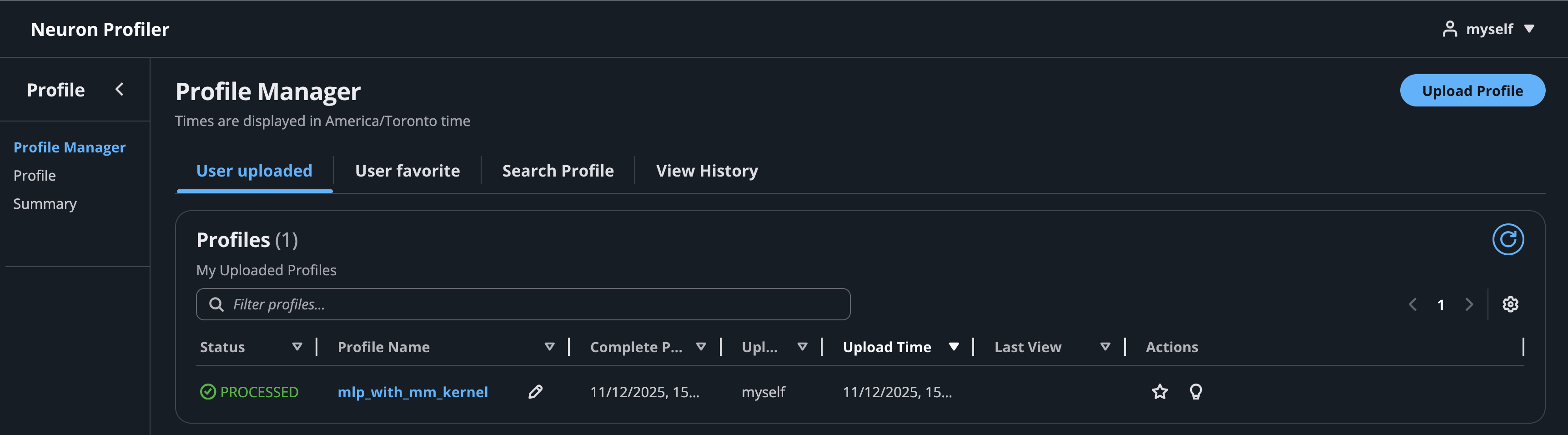
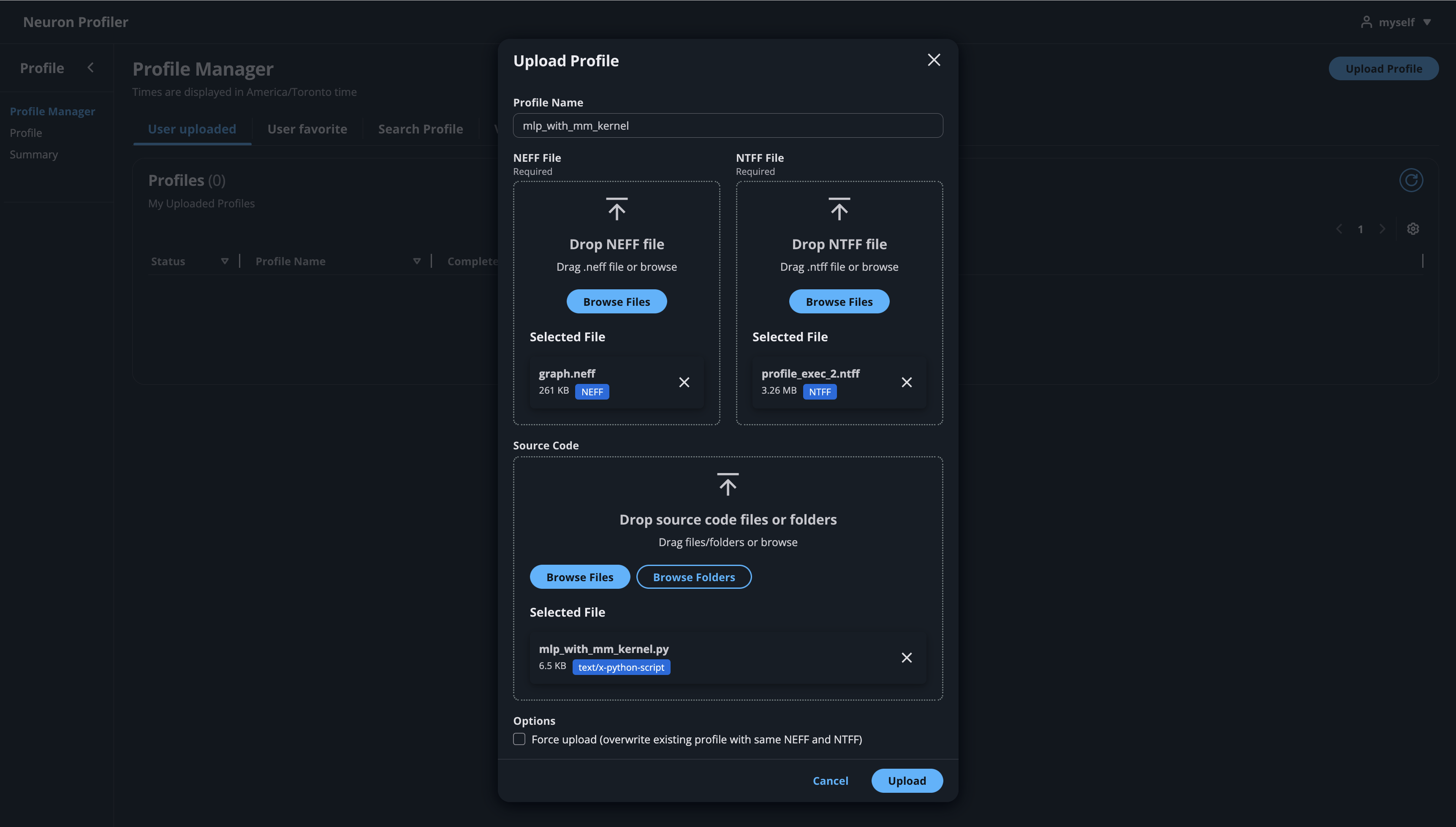
Click on the button “Upload Profile” to upload NEFF and NTFF files, and give a meaningful name to your profile. It is optional to select source code folder for code linking.
After the files are uploaded and processed, you will be able to open the profile from the list.

If you click on the name of your profile in Profile Name column, it will navigate to profile page
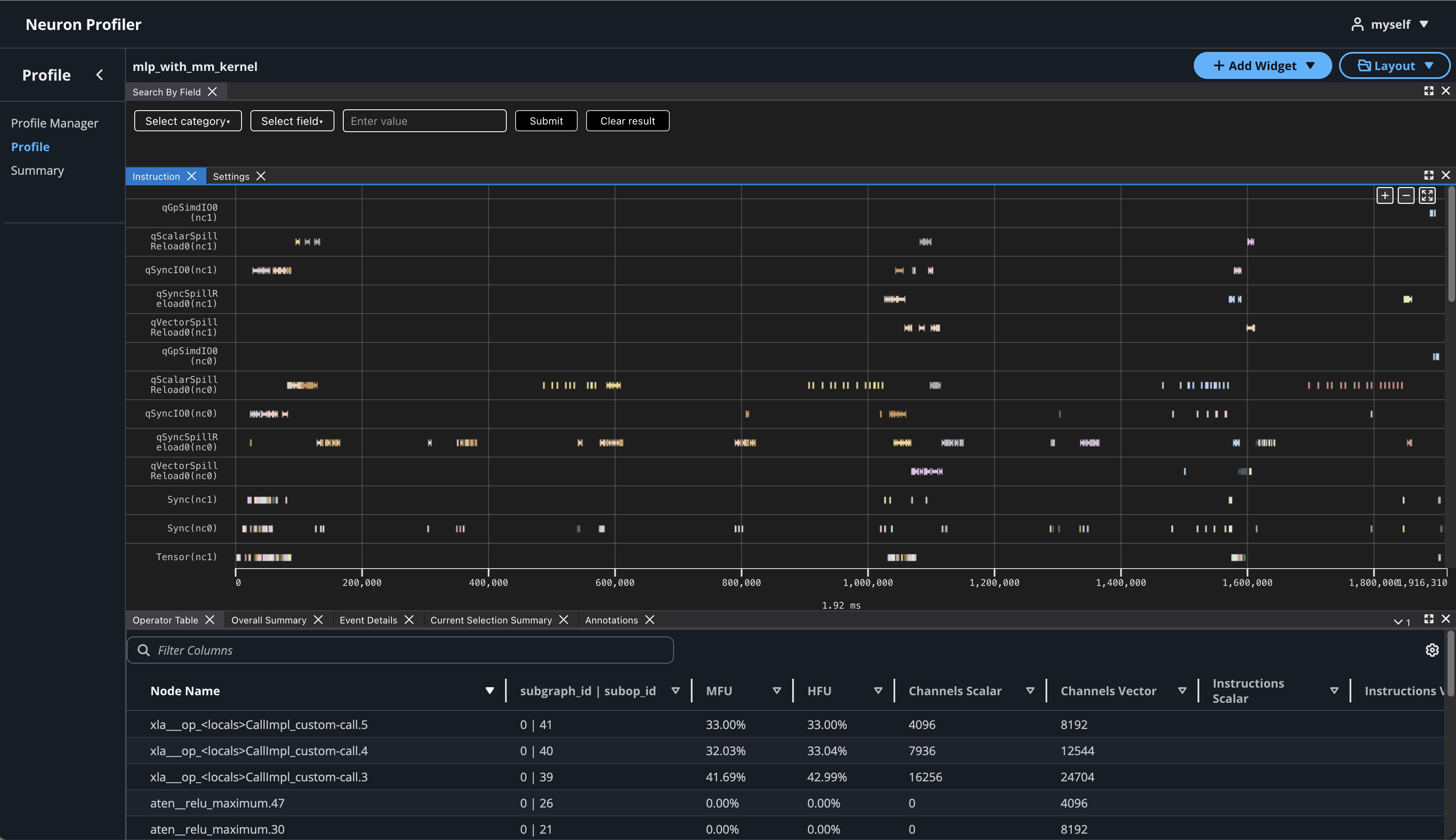
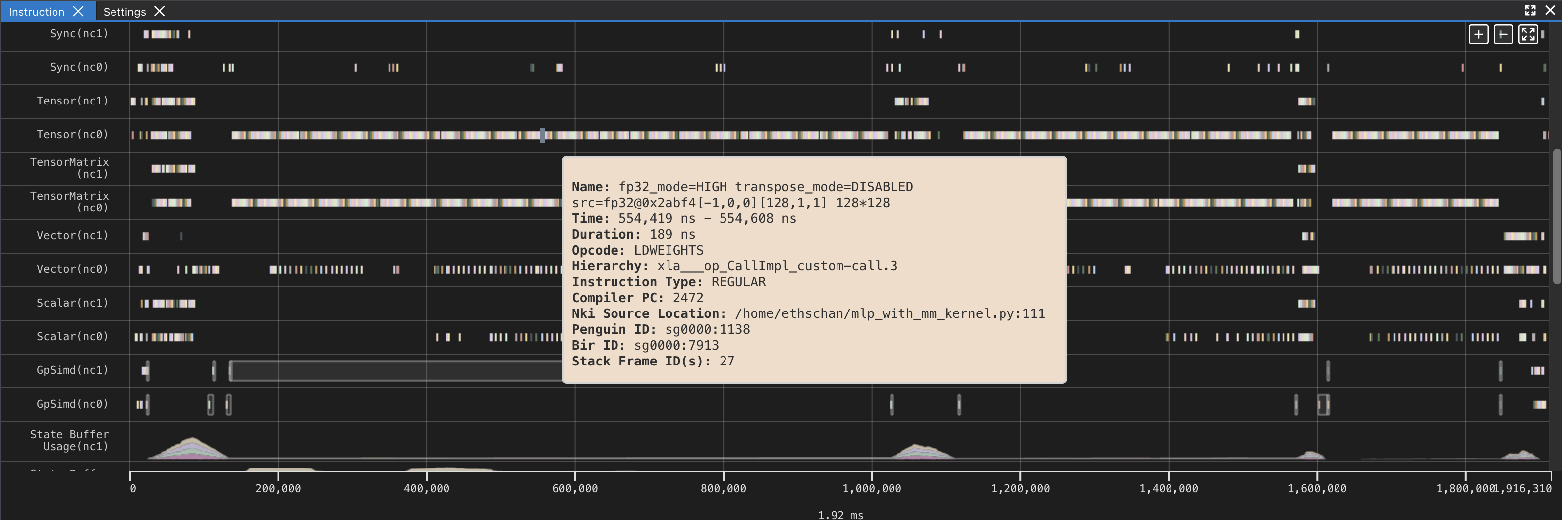
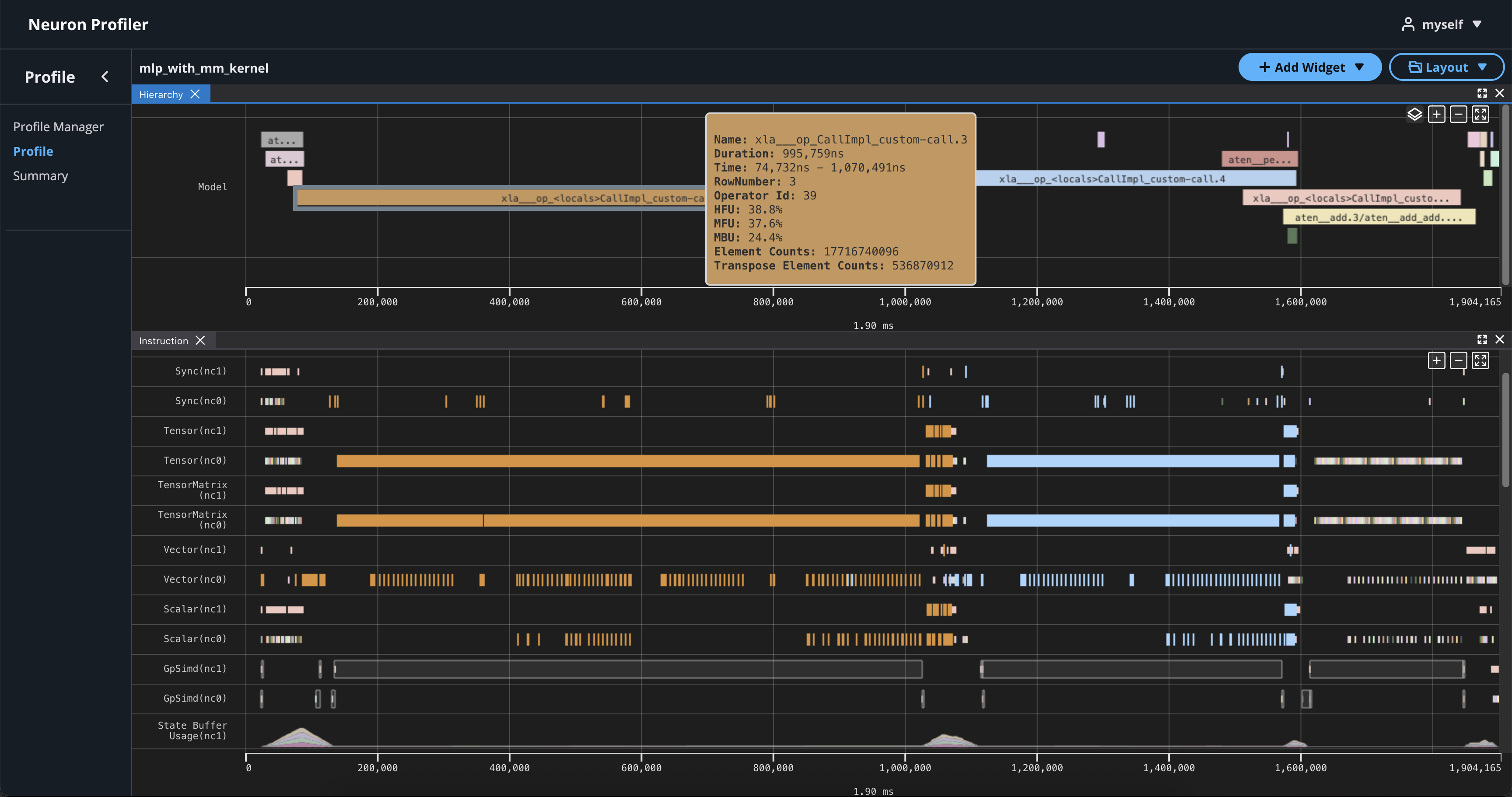
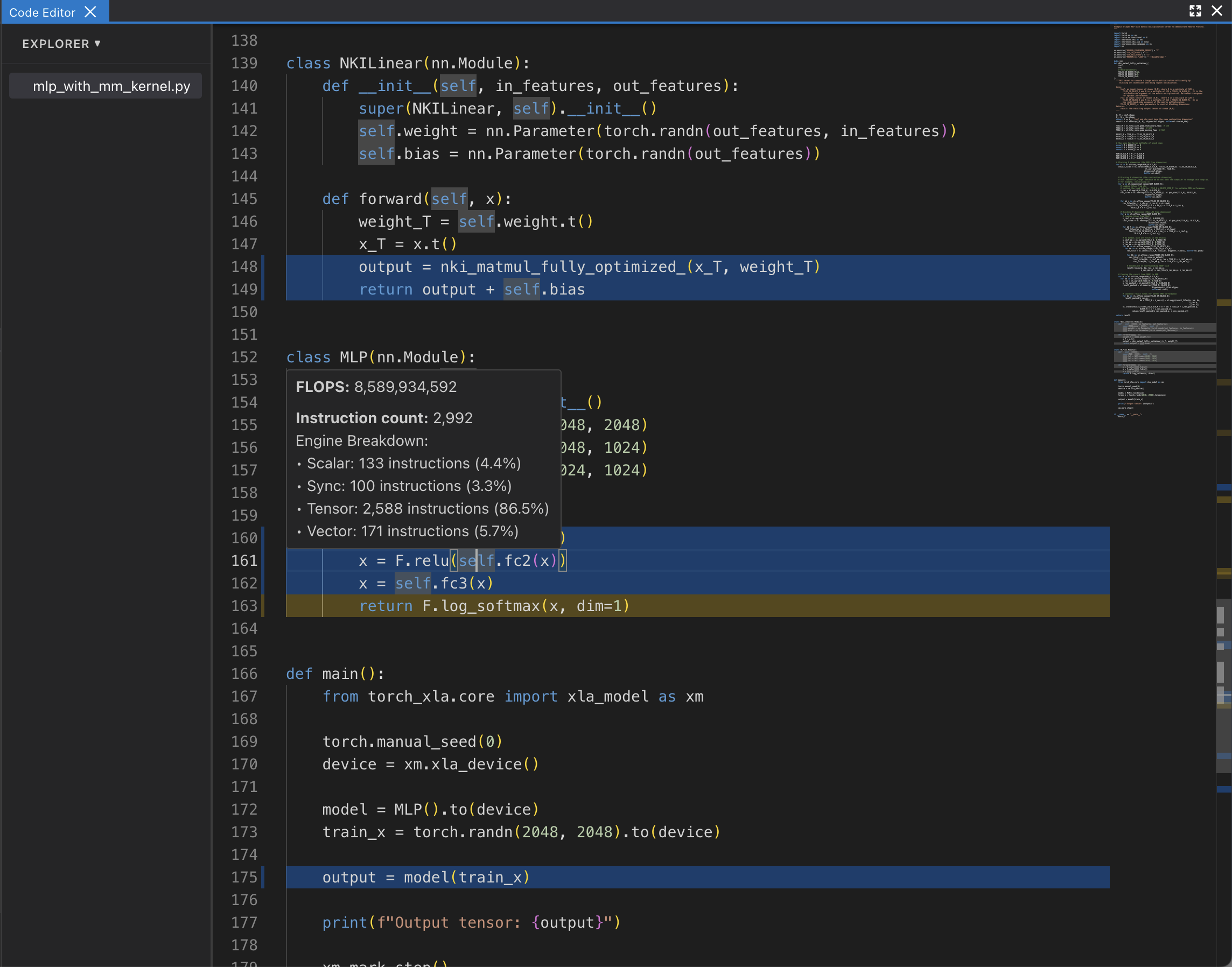
If you hover over any engine instruction in the timeline with your mouse, you will see instruction details in a pop-up box.
If you click on any engine instruction in the timeline with your mouse, you will see event details in a panel below the timeline.

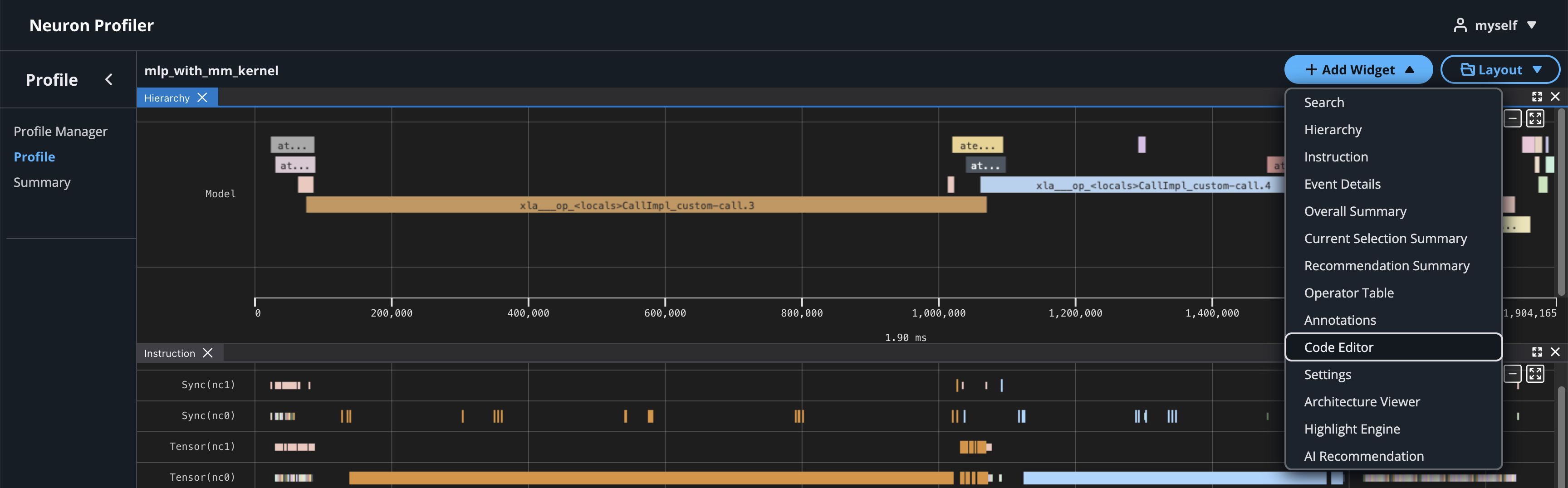
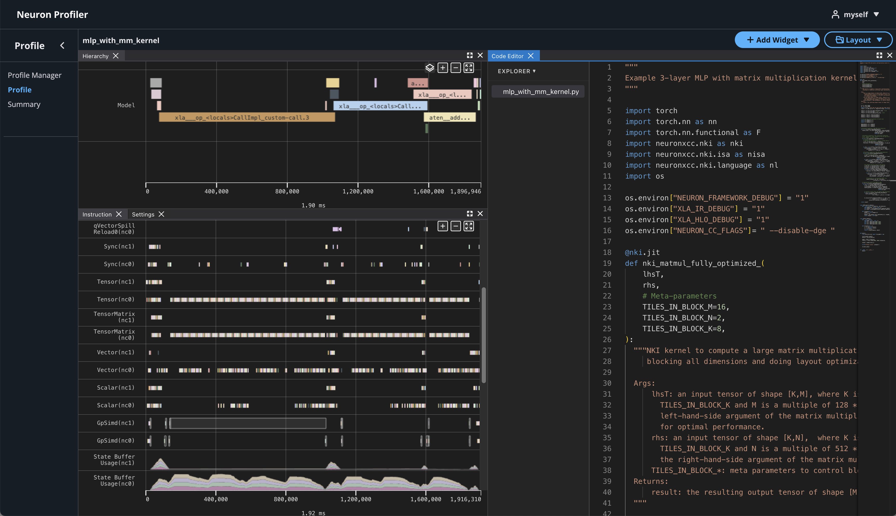
To view hierarchy of this profile, click on Add Widget and select Hierarchy.
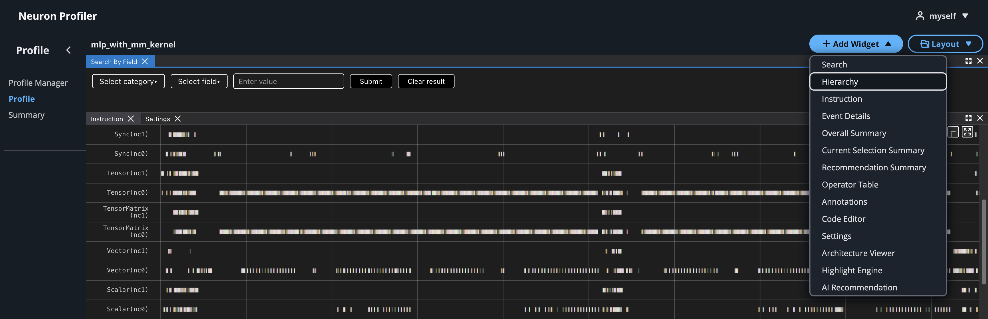
Using the Profiler’s flexible layout support, you can drag and group every widget into any panel of your choice to customize the layout for your workflow.
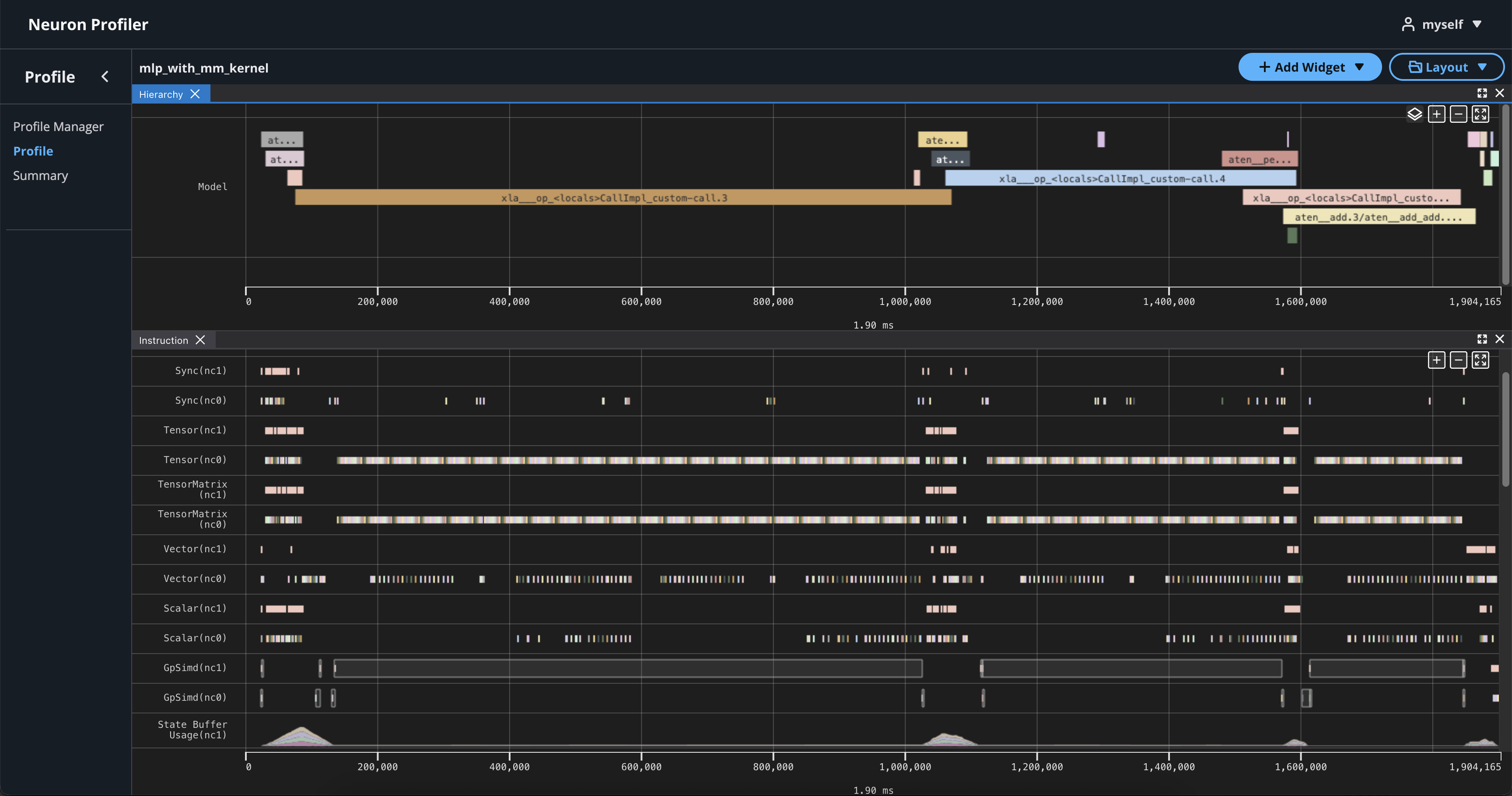
If you right-click on an operator in the hierarchy timeline, it will highlight all related instructions in the instruction timeline.
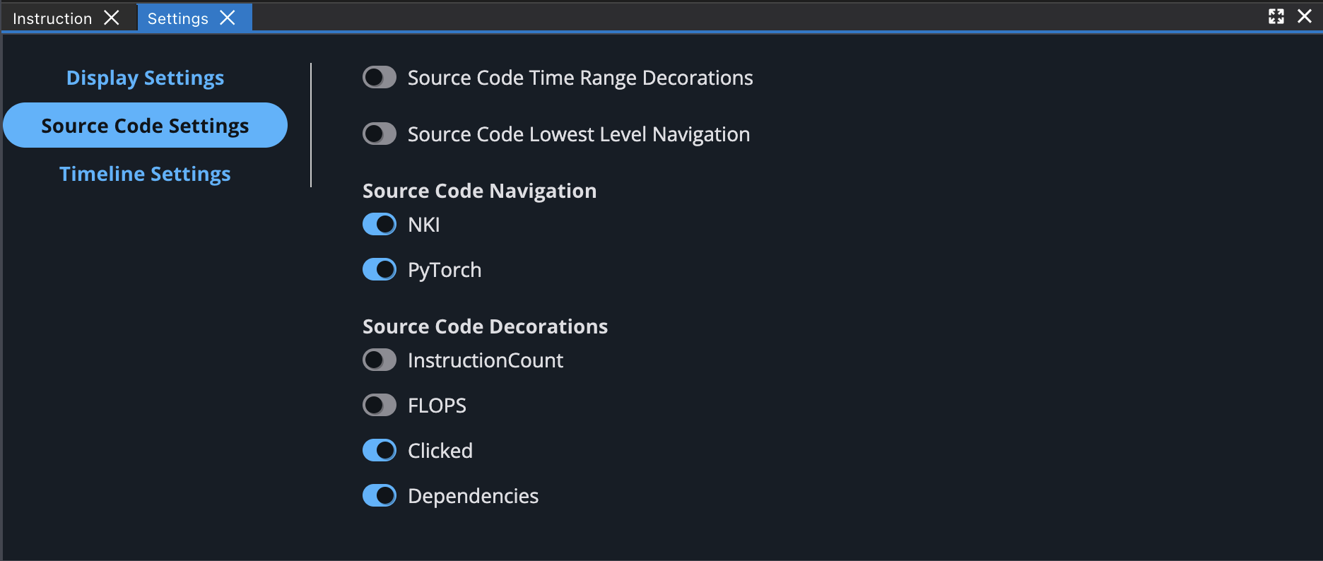
View NKI Source Code in Neuron Profile#
You can optionally include your NKI source code files for display in Neuron Profile. When provided, Neuron Profile loads the source code into an integrated viewer, displayed side-by-side with the execution timeline in the web UI. This makes it easier to navigate between the instruction trace and the corresponding NKI source code, and to track the exact version of the code that generated the profile.
Note
Even if you don’t upload the source code, the NKI source filename and line number remain available in the instruction detail view as noted in View Neuron Profile UI.
If source code is uploaded with NEFF and NTFF file, you will be able to see the source code in the code editor. To open the code editor, click on Add Widget and select Code Editor.
The code editor will be open on the right hand side.
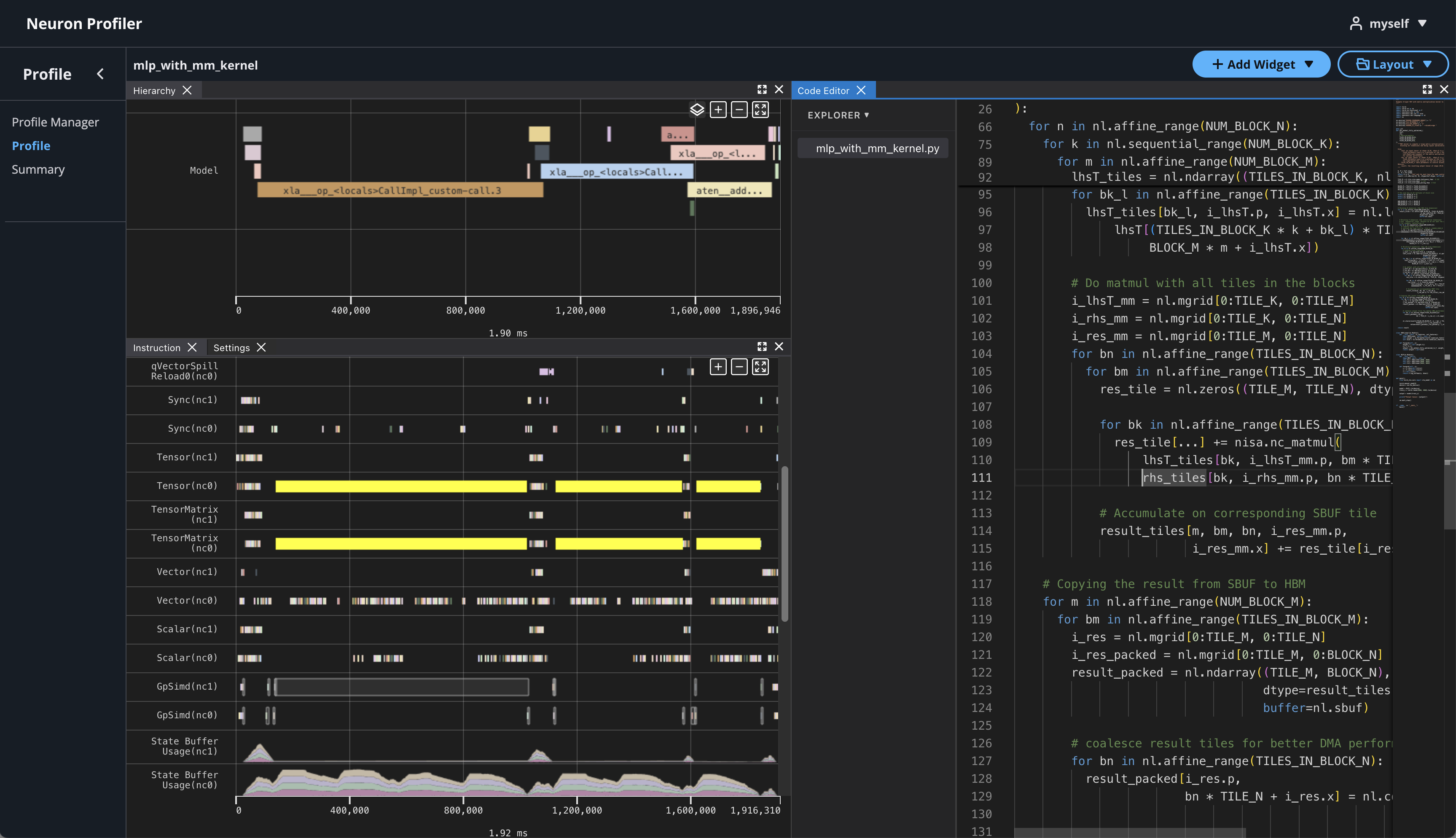
Hover on an instruction that has NKI source location and Command + left click on Mac (Control + right click on Windows), it will pop-up a window for showing file selection for stack trace.
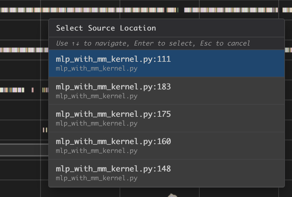
Selecting any option from the list, it will jump to the line of the source code and highlight all of instructions related to this line.
You can also enable different source code decorations in Source Code Settings.
Next Steps#
Great! Now that you’ve learned how to profile an NKI kernel, it’s time to take this further:
Dive into the NKI Performance Guide to discover techniques for making your kernels faster and more efficient.
Explore the NKI sample kernels to see real-world examples of high-performance kernel implementations — and get inspiration for your own NKI kernels.
By combining profiling insights with optimization strategies and practical examples, you’ll be well-equipped to write NKI kernels that leverage Neuron hardware in an efficient way.