This document is relevant for: Inf2, Trn1, Trn1n

NKI Performance Guide

In this document, we describe a recipe to find performance bottlenecks of NKI kernels and apply common software optimizations to address such bottlenecks. During this process, we will showcase how to leverage neuron-profile, a GUI-based performance profiler designed for NeuronDevices, to guide your performance optimization efforts. Before proceeding with this document, please make sure to read through Trainium/Inferentia2 Architecture Guide to familiarize yourself with Neuron hardware architecture.

Ideally, performance optimization efforts would end with one of two possible outcomes: the execution of a NKI kernel is either strictly compute-bound or memory-bound. In the context of NeuronDevices, compute-bound means at least one of the compute engines is active close to 100% of the kernel execution time (90%+ is considered good in practice), while memory-bound typically means the achieved device memory bandwidth utilization (MBU) is close to 100% (60%+ is considered good in practice). For compute-bound kernels that are matrix-multiplication dominated, we should also aim for close to 100% model flops utilization (MFU) in the execution. All of these metrics are available under the Summary tab in neuron-profile GUI:

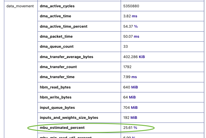
Fig. 41 MBU metric in neuron-profile.

Fig. 42 Compute-related metrics in neuron-profile.

The rest of this document is divided into three sections, focusing on three categories of performance optimizations. The first section covers optimizations to maximize achieved arithmetic intensity, with the goal of minimizing compute engine idle periods due to unnecessary data movement. The second and third sections dive into optimizations to improve compute engine and data movement efficiency, respectively.

Improving Arithmetic Intensity

Arithmetic intensity of a computation workload is commonly defined as the average number of computation operations performed per byte of data accessed from memory. In the context of NeuronDevices, the definition refers to data accessed from device memory (HBM), since the on-chip memory (SBUF) has sufficient bandwidth to keep all compute engines busy.

When arithmetic intensity is overly low, compute engines would be consuming data much faster than DMA engines fetching data from device memory into the on-chip memory SBUF. In this case, the execution is bounded by the available device memory bandwidth. Once arithmetic intensity is beyond certain threshold, that is, ratio of maximum compute throughput over memory bandwidth, the performance bottleneck shifts to how fast compute engines can perform computation, which leads to a compute-bound execution.

Figure below visualizes the Roofline Model, which captures this idea by plotting the projected attainable compute throughput with respective to the arithmetic intensity of an algorithm.

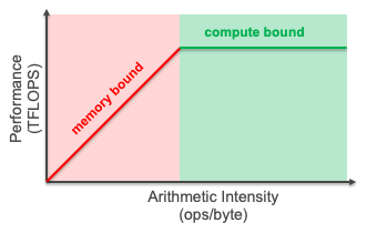
Fig. 43 The Roofline Model.

Algorithmic arithmetic intensity is an intrinsic characteristic of the particular workload and solely dependent on the compute algorithm. In reality, due to limited capacity in SBUF, the achieved arithmetic intensity of a NKI kernel implementation of such workload could be lower than the algorithmic arithmetic intensity. This could lead to excessive compute engine idle time blocked by completion of data movements. The two typical reasons behind this are input data reloading and intermediate data spillage. Let’s discuss how to identify their symptoms in neuron-profile and how to mitigate these issues to improve arithmetic intensity next.

Opt #1. Exploit temporal locality to minimize input data reloading

Symptom: In neuron-profile, if a NKI kernel triggers DMAs (nl.load) for the same input tensor multiple times, you would see the relevant DMA activities (on the timeline row with a label starting with q and ending with IO) being highlighted in an orange box. Hovering over the “+” sign of the box in top-left corner, a performance warning pop-up will show up, indicating which input tensor is being reloaded, the size of it and how many times it was reloaded. For example, figure below is a screenshot of such warning pop-up showing the u input tensor defined in my NKI kernel was reloaded ~7 times:

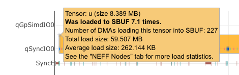
Fig. 44 Performance warning on input data reloading.

Optimization: Input tensor reloading could be avoided if the same data stay in SBUF across all the operations that consume it at different points of the execution. However, keeping too much data in SBUF across operations can increase the memory pressure in SBUF, leading to more spilling of intermediate data. Therefore, avoiding input reload should be a trade-off programmers need to make carefully. Figure below illustrates this trade-off conceptually.

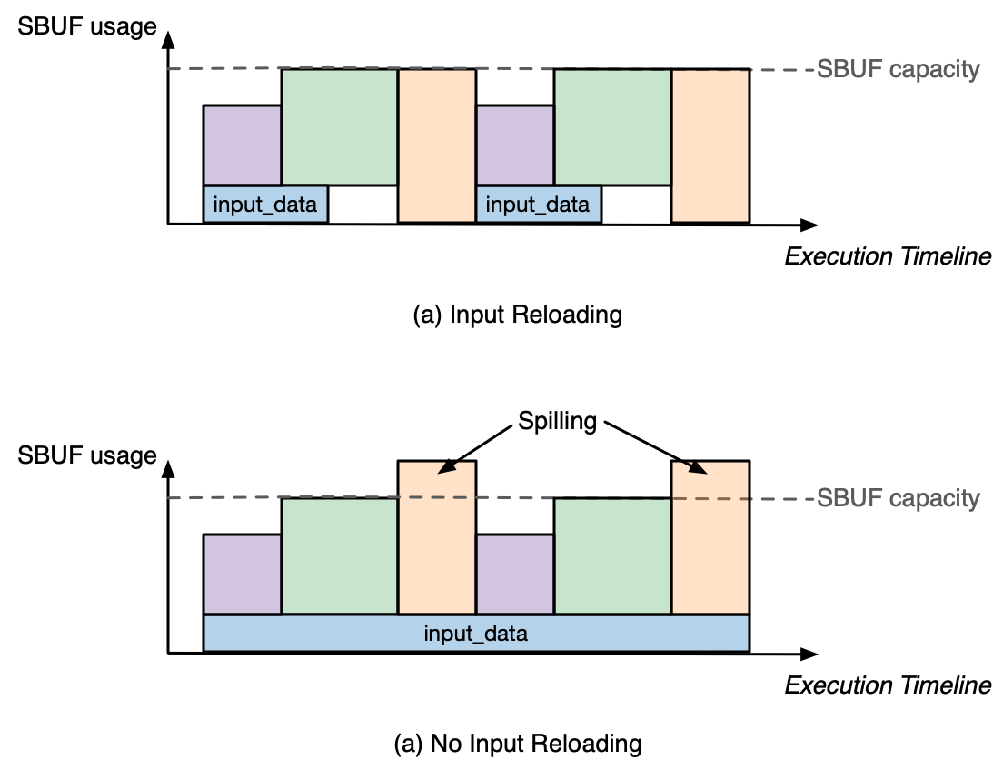
Fig. 45 SBUF usage impact with and without input reloading.

A classic example of using this optimization technique is in a matrix multiplication kernel, where we need to exploit data reuse in the same rows of the left hand-side input matrix across different columns of the right hand-side matrix. See Matmul NKI Tutorial Optimization 1-3 for more detailed discussion. Another great example is in the Fused Mamba kernel tutorial, where programmers can minimize reloading of largest input tensors through loop reordering.

Opt #2. Fuse operations to minimize intermediate data spilling

Symptom: In neuron-profile , we can find many useful data movement related metrics in the Summary tab:

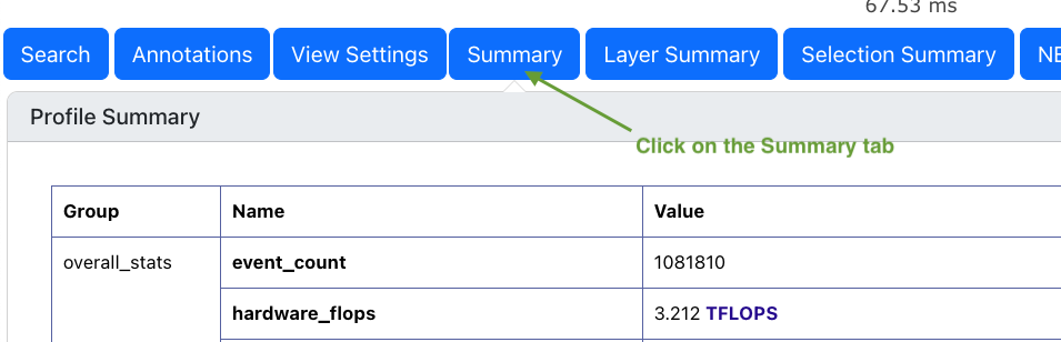
Fig. 46 neuron-profile Summary tab.

Below we highlight four relevant metrics to assess severity of data spilling under the data_movement section (tip: hovering over any metric name will show a detailed description of the metric):

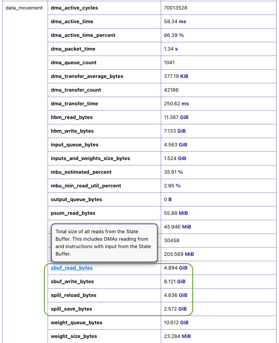
Fig. 47 Data movement metrics

Here, spill_save_bytes refers to the total size of intermediate data in bytes the workload spills from SBUF into device memory, while spill_reload_bytes indicates total size of spilled data in bytes the workload reloads back into SBUF. By comparing spill_save_bytes against sb_read_bytes, you can get a feel on how much of the data movement traffic from SBUF to device memory is related to spilling. Similarly, comparing spill_reload_bytes against sb_write_bytes indicates how much of traffic from device memory back to SBUF is related to spilling. If the spill related traffic takes up a significant portion (for example over 30%), it is likely worthwhile to take a close look at this optimization.

Optimization: To reduce spilling, the key is to find operator fusion opportunities in the kernel. To achieve fusion, we typically also need to slice up computation of each operator and perform computation for a portion of the input tensor at a time. As a simple example, assume a chain of operators op0 → op1 on a large input tensor kernel_in_hbm that cannot fit in SBUF all at once. If we were to do the operators one at a time, we will effectively have the following sequence of events:

for tile in kernel_in_hbm:
    tile_sbuf = load(tile)
    op0_out_sbuf = op0(tile_sbuf)
    # compiler generated spilling, or NKI programmers explicitly perform a store
    spill_save(op0_out_sbuf, op0_out_hbm)

for tile in op1_out_device_memory:
    tile_sbuf = spill_reload(tile)
    op1_out_sbuf = op1(tile_sbuf)
    store(op1_out_sbuf, kernel_out_hbm)

However, if we fuse the operators from above:

for tile in kernel_in_hbm:
    tile_sbuf = load(tile)
    op0_out_sbuf = op0(tile_sbuf)
    op1_out_sbuf = op1(op0_out_sbuf)
    store(op1_out_sbuf, kernel_out_hbm)

Inside a NKI kernel, operator fusion is exactly done as the above through explicit loop fusion.

One great use of this optimization is the self attention operator commonly found in Transformer models. Self attention performs a chain of operators: matmul_0 → softmax → matmul_1, where matmul_0 of a single attention head produces a large intermediate tensor shape that overflows SBUF in common Transformer models with a context length in the thousands. See Fused Attention Tutorial for more detailed discussion.

Optimization Gotchas: Certain code patterns in NKI might lead to unexpected spilling from programmers’ perspectives. We are working on improving these in future releases. As an example, buffers sometimes need to be declared within the inner loop to avoid spilling. In other words, instead of:

buf = nl.ndarray((2, 4, nl.par_dim(128), 512), buffer=nl.sbuf)
for i0 in nl.affine_range(2):
  for i1 in nl.affine_range(4):
     buf[i0, i1, ....] = nl.load(...)
     ...

we need to implement:

for i0 in nl.affine_range(2):
  for i1 in nl.affine_range(4):
     buf = nl.ndarray((nl.par_dim(128), 512), buffer=nl.sbuf)
     buf[...] = nl.load(...)

With the above aforementioned optimizations, the kernel execution should achieve an arithmetic intensity that is somewhat close to the algorithmic arithmetic intensity. At this point, you should be able to observe from the execution timeline in neuron-profile whether the kernel spends more time in compute or DMA engines. The engine/dma_active_time_percent metrics reported in the Summary tab should also give you good hints. If your kernel execution is dominated by computation, we recommend going over Optimizing Compute Efficiency first to optimize compute efficiency. Otherwise, jump straight to Optimizing Data Movement Efficiency to understand how to optimize data movement efficiency.

Optimizing Compute Efficiency

Compute efficiency optimizations typically fall into two categories:

1. “time” domain engine utilization: reduce engine idle time to keep the compute engine on critical path as busy as possible, such as enabling pipelining among engines.

2. “spatial” domain engine utilization: within the engine active periods, increase instruction efficiency to use as many hardware units within the engine as possible, such as combining multiple instructions into one.

Let’s dive into each category below.

Reducing engine idle time

To improve the active time of a compute engine, we need to understand the exact reasons for the engine to enter an idle state. In neuron-profile, we can focus on the execution trace of the bottlenecked engine and zoom into the visually large engine idle gaps. For example, in the below profile, we expect VectorE to be the bottlenecked engine and therefore focus on the idle gaps on VectorE:

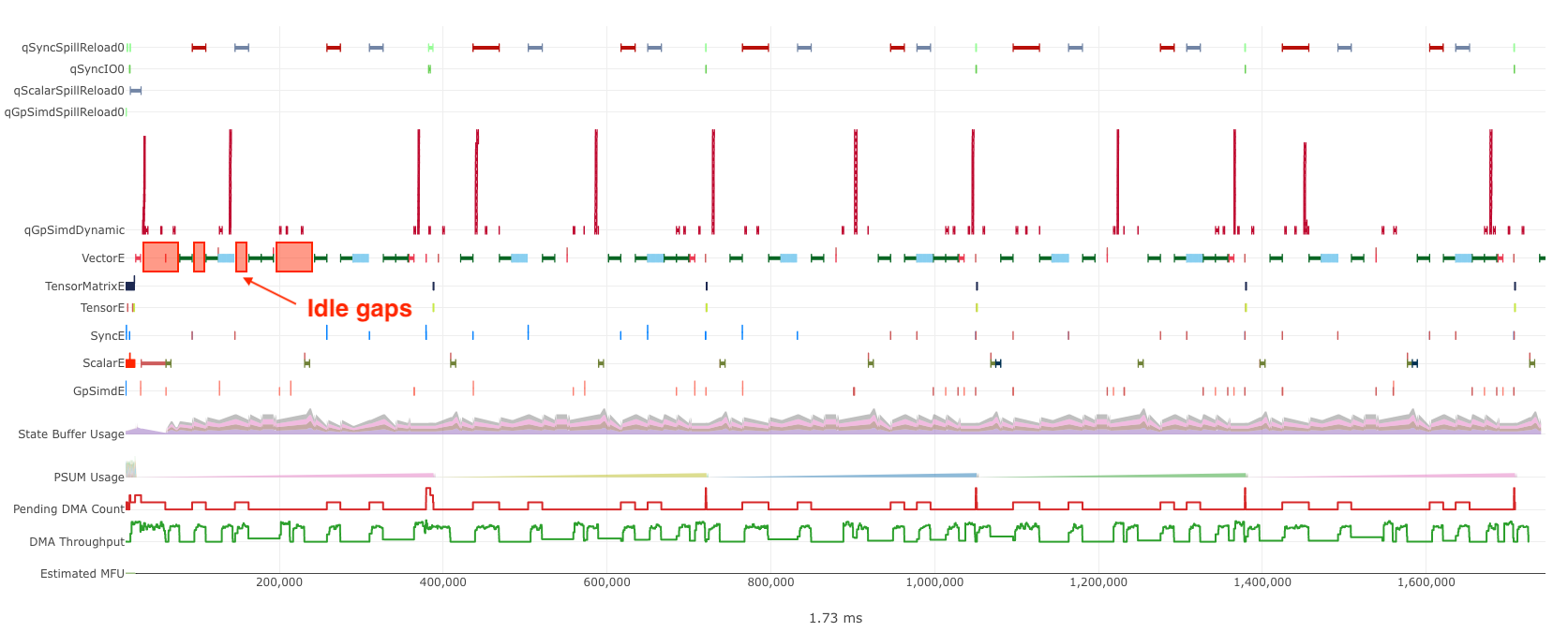
Fig. 48 Engine idle gaps.

Side note, for faster GUI rendering, neuron-profile enables data sampling by default and “hides” certain instructions from the timeline with a large profile. To confirm whether an engine indeed has an idle gap, we recommend zooming into a smaller region of the profile and turn on “Show unsampled data” in View Edit Settings to make sure all instructions are rendered:

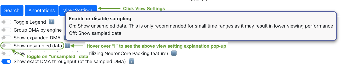
Fig. 49 Show unsampled data in neuron-profile.

For each engine idle gap, you can find out the reasons why the engine cannot execute instructions by inspecting the semaphore wait condition of the first instruction executed on the engine after the gap. Broadly speaking, these semaphore wait conditions are either waiting for 1) other compute engine instructions or 2) DMA activities to finish. We have different techniques to shrink the idle gaps caused by either of these wait conditions (that is, engine stall reasons).

Opt #3. Overlap execution across compute engines through pipelining

Symptom: The semaphore wait condition of the first instruction after an idle gap is on a semaphore name that matches a compute engine name in NeuronCore: Vector, Scalar, GpSimd and Tensor. These semaphores are associated with instruction completion on the corresponding compute engine.

For example, the below TENSOR_TENSOR instruction on VectorE is waiting for S[4] (Scalar) to reach a value of 36. This means VectorE was waiting for ScalarE to finish certain instructions.

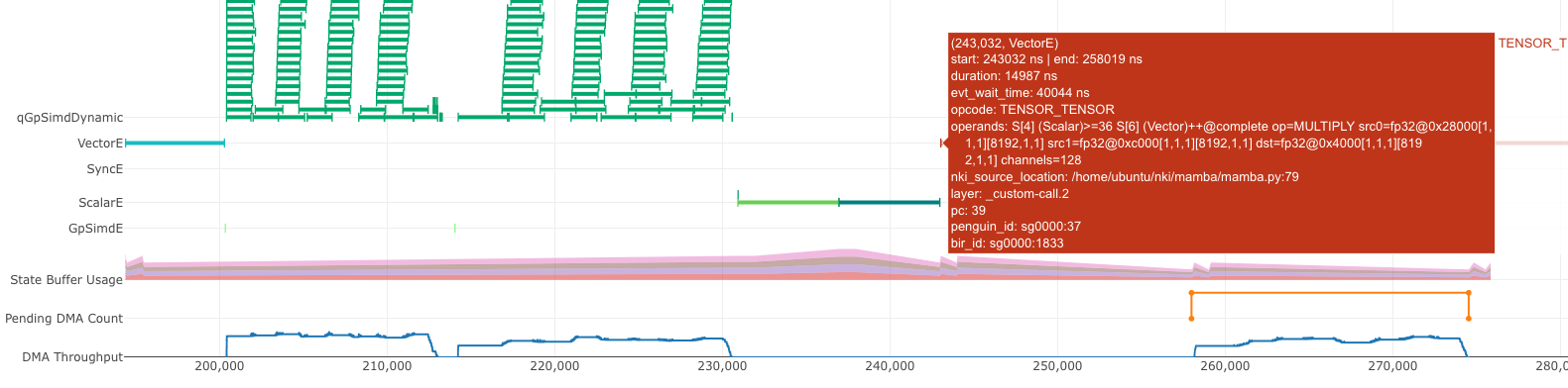
Fig. 50 Semaphore wait on another compute engine.

Optimization: When there is a sequence of operators on different compute engines, we can slice the computation in a way that the compute engines can process tiles of the original operator in a pipeline fashion. As an example, let’s assume we have two operator back to back on a large (say, thousands of elements) tensor X: X → op0 → Y → op1 → Z. op0 is performed on ScalarE while op1 is on VectorE. For simplicity, let’s assume tensor X/Y/Z have the same shape.

Figure below shows two possible execution timelines with and without engine pipelining. Without pipelining, VectorE is fully idle when ScalarE is executing op0 on tensor X in the first half of the execution. Similarly, ScalarE is idle while VectorE is running op1. However, with pipelining, ScalarE is able to produce partial results in tiles and unblock VectorE as soon as the first tile is processed. Overall, engine pipelining shortens the end to end latency to complete op0 and op1, through shrinking engine idle time and improving hardware utilization.

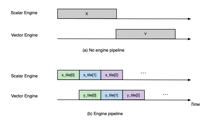
Fig. 51 Engine timeline with and without engine pipelining.

Choosing a proper tile size is crucial to the performance of such engine pipelining. It is up to NKI programmers to make this choice in kernel implementation and iterate on it using performance profiling data in neuron-profile. For complex kernels, we often need to schedule a pipeline among all engines: Tensor/Scalar/Vector/GpSimd Engine.

For example, in Transformer’s self-attention layer, in addition to fusing matmul_0(Q, K) → softmax → matmul_1(softmax_out, V) in a single kernel to minimize spilling as discussed in Opt #2, we also need to form a complex engine pipeline for the operators to maximize utilization of the compute engines:

• matmul_0/matmul_1: TensorE

• softmax:

  • exponential: ScalarE

  • summation: VectorE

  • scale by reciprocal of summation: ScalarE

  • for causal self attention, triangular masking: GpSimdE

See Fused Self Attention tutorial for more detailed discussion.

Opt #4. Overlap data loading with computation

Symptom: The semaphore wait condition of the first instruction after an idle gap is on a semaphore name that starts with letter q. These semaphores are associated with completion of DMA activities.

For example, hovering on an instruction will bring up the key instruction details as follows:

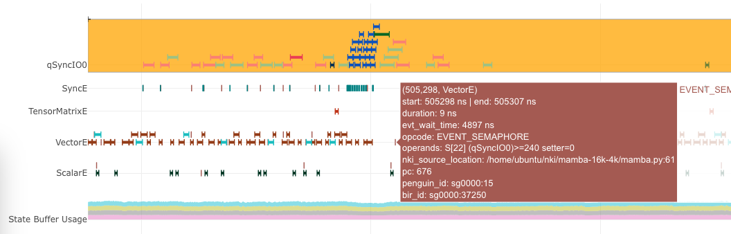
Fig. 52 Instruction waiting for input data loading.

In this particular screenshot, the EVENT_SEMAPHORE instruction could not start earlier even though VectorE was idle because it was waiting for semaphore S[22] (qSyncIO0) to reach a value of 240. The semaphore is only incremented whenever the corresponding DMA activities shown on the qSyncIO0 execution trace are completed. Clicking on the DMA activities on qSyncIO0 immediately before the EVENT_SEMAPHORE instruction, you may follow the nki_source_location to find out which line of code is related to this DMA activity (nl.load() call).

Similarly, if an instruction is blocked on S[47] (qSyncSpillReload0), that means it is blocked by DMA activities for spilling:

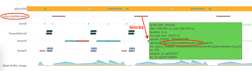
Fig. 53 Instruction waiting for spilled data reloading.

Clicking on the DMA activities on qSyncSpillReload0 immediately before the EVENT_SEMAPHORE instruction, you may find out the name of the intermediate NKI tensor that was spilled/reloaded. For example, the below DMA transfer reloads the tensor named deltaU as defined in our NKI kernel. Note, spill/reload DMA transfers are generated by Neuron Compiler automatically by analyzing SBUF usage in NKI kernels. Therefore, these DMA transfers do not have an associated explicit NKI API call or nki_source_location information.

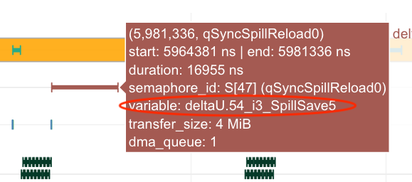
Fig. 54 Spilled tensor variable name.

Optimization: Overlapping data loading with compute is highly similar to enabling compute engine pipelining in Opt #3, since DMA engines can move data in parallel to compute engine execution, just like how compute engines can run different operators in parallel.

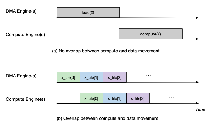
Fig. 55 DMA and engine timeline with and without overlapping.

However, it is also possible that even after maximizing overlapping of compute and data movement the best you can, the data movement duration is still not hidden behind compute even though your kernel has a compute-bound arithmetic intensity. In these cases, the most common cause is the data movement in your kernel is not using the DMA engines efficiently. Refer to a later section to see relevant optimization techniques to improve DMA bandwidth utilization.

As a concrete example, we demonstrate how to properly overlap compute and data movement in a compute-bound (VectorE as the bottlenecked engine) kernel in Mamba tutorial.

Improving engine efficiency

Once done with “avoiding engine idle gaps” as much as possible, we can focus on improving “engine efficiency” during the busy periods of the engine. We will start with two optimizations techniques that are generally applicable to all compute engines, followed by TensorE-specific optimization techniques.

Opt #5a: Use sufficiently large input tiles in free dimension

Symptom: Certain operators might trigger many back-to-back instructions with small free dimension sizes in the input tensors. For example, in the below profile, ScalarE is busy with many repeated activation instructions with IDENTITY (scale/bias enabled) activation function, which is equivalent to calling nki.isa.tensor_scalar(op0=nl.multiply, op1=add) APIs. If you click on one of the instructions to pull up the instruction detailed view, you can see the source tensor access pattern is fp32@20580[1,1,1][1,1,1] , where the first set of bracket indicates 3D strides and the second set indicates 3D shape in FP32 elements. More detailed discussion of ISA access pattern can be found by clicking on the i button at the end of the Operands row.

In this example, each of the back-to-back instructions is reading one element per partition from SBUF, which would take about one engine cycle to perform useful computation within the instruction. Such instructions are extremely inefficient since the static instruction overhead in the order of ~100 cycles would be limiting the overall throughput.

To make things worse, these instructions also have data dependency (read after write) between consecutive instructions, which means the next instruction cannot start data read until the previous instruction has all of its output committed to the local SRAM. In neuron-profile, you can inspect data dependency between instructions by clicking on an instruction of interests (Inst1 in the below profile), which will highlight the clicked instruction and also the instruction that produces input for the clicked instruction (Inst0 in the below profile). The dependency information can also be viewed in the details “instruction dependency pcs”. In fact, all the neighboring instructions also have a similar dependency patterns in this profile.

With the above inefficiencies, the initiation interval (the time between the starting points of two consecutive instructions) for these instructions on ScalarE is around 189 ns (264 ScalarE cycles on NC-v2) , which is much higher than the useful computation cost (one ScalarE cycle throughput-wise).

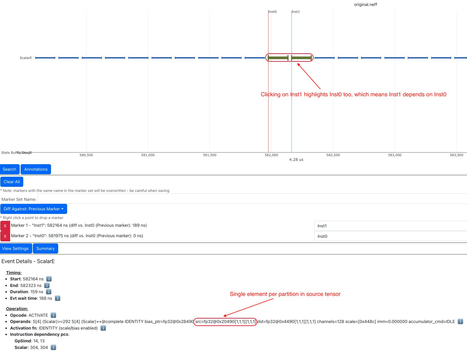
Fig. 56 Many back-to-back ScalarE instructions with small tensor shapes

Optimization: The trick of this optimization is to increase the free dimension size of instruction input tiles. As discussed in the architecture guide, NeuronCore compute engines typically require at least 128 elements/partition in the source tensor to be efficient. However, it is worth mentioning that increasing free dimension sizes might not be trivial due to the high-level computation definition. We suggest developers walking through the architecture guide in detail to better understand capabilities of different compute engines, and mapping/reformulating the high-level operators onto the engines using the most suitable instructions. Such instructions could be invoked either through the high-level [nki.lanaguage](api/nki.language.html) or low-level [nki.isa](api/nki.isa.html) APIs.

In addition, keep in mind there is a trade-off in choosing the free dimension size in instruction input tiles: Too small of a tile size exposes significant instruction overhead leading to inefficient engine execution, while too large of a tile size often leads to inefficient pipelining between engines (working against Opt #3) and high memory pressure in SBUF (working against Opt #2).

As an example, a naive implementation of the prefix sum scan operation in Mamba v1 would trigger seq_len back-to-back single element nki.isa.tensor_scalar instructions as shown in the above profile example, where seq_len is the sequence length of the model typically in the range of thousands. A more efficient way to implement this operation is through a special VectorE instruction nisa.tensor_tensor_scan. See the Mamba tutorial <tutorials/fused_mamba> for more discussion.

Opt #5b: Use sufficiently large input tiles in partition dimension

Symptom: When instructions use input/output tiles that span fewer than 128 partitions, they typically under-utilize the compute engine capabilities. This is because each SBUF/PSUM partition has a one-to-one mapping to parallel vector lanes in the compute engines. As an example, the TENSOR_TENSOR instruction (equivalent to nki.tensor_tensor) on VectorE takes a source tensor in SBUF that occupies 64 partitions only, as indicated by the channels=64 instruction operand field. If we were to increase the channels field to 128, the instruction would have taken the same amount of time as channels=64.

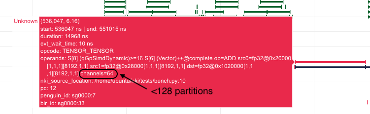
Fig. 57 An instruction that read/write less than 128 partitions.

Similarly, for a MultiplyMoving instruction (Matmul opcode in neuron-profile) TensorE, if the instruction reads/writes tiles do not span the full SBUF/PSUM partitions, we would be underutilizing TensorE. As an example, the below MultiplyMoving instruction only writes to 96 partitions in PSUM, as indicated by the operand 128*96, which means the instruction only uses 128 rows and 96 columns of the processing elements out of the available 128x128 systolic array.

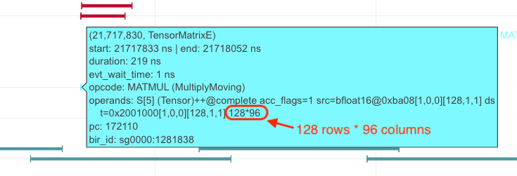
Fig. 58 MultiplyMoving instruction that uses <128 TensorE columns

Optimization: If we see many back-to-back instructions on the compute engine that have fewer than 128 partitions in the input/output tiles as discussed above, we should consider an optimization called “partition vectorization”.

As an example, say we have two nki.isa.nc_matmul() instructions with each generating a 64-partition PSUM tile of the same shape. Then VectorE needs to run nki.isa.tensor_reduce() on both tiles to generate a reduction result. Note, on trn1/inf2, VectorE cannot run the two independent nki.isa.tensor_reduce() instructions in parallel in this case, even though the total number of compute lanes required for these instructions does not exceed 128. To improve VectorE utilization in this case, we can:

1. The two nc_matmul() instructions write to disjoint PSUM partitions: partition 0-63 for the first nc_matmul and partition 64-127 for the second one.

2. Invoke a single nki.isa.tensor_reduce() instruction to process output of both nki.isa.nc_matmul() instructions.

The below pseudo-code illustrates the above computation without and with partition vectorization.

import neuronxcc.nki.isa as nisa
import neuronxcc.nki.language as nl

################################################################
# option 1: No partition vectorization
# two 64-partition vector instructions running serially

# By default, NKI creates mm_tile0 and mm_tile1 in partition 0-63
mm_tile0 = nisa.nc_matmul(...)
mm_tile1 = nisa.nc_matmul(...)

# Both nki.isa.reduce instructions move data from psum partition 0-63
# in a serialized fashion
reduce0 = nisa.tensor_reduce(mm_tile0, ...)
reduce1 = nisa.tensor_reduce(mm_tile1, ...)

################################################################
# option 2: Partition vectorization
# vectorized into one 128-partition vector instructions

# Here, we explicitly declare a 128-partition tensor in PSUM
mm_tile = nl.zeros((128, ...), np.float32, buffer=nl.psum)

i_output0_p = nl.arange(64)[:, None]
i_output1_p = 64 + nl.arange(64)[:, None]
# Assign first part of mm_tile to partition 0-63
mm_tile[i_output0_p, ...] = nki.isa.nc_matmul(...)
# Assign second part of mm_tile to partition 64-127
mm_tile[i_output1_p, ...] = nki.isa.nc_matmul(...)

# A single nki.isa.reduce instruction, using all 128 partitions
reduce = nisa.tensor_reduce(mm_tile, ...)

Option #2 above is able to perform the reduction 2x faster, by vectorizing the partition dimension and performing a single reduction instead of two.

Opt #6: Combine instructions

Symptom: Even though the majority of popular ML models are matrix multiplication heavy, certain operators can be vector/scalar operation heavy instead, such as self-attention in Transformer models. These operators typically have a performance bottleneck in VectorE or ScalarE or both. As an example, the below profile shows the inner loop of self attention, where either VectorE or ScalarE is busy at any moment in time, while TensorE has clear engine idle gaps.

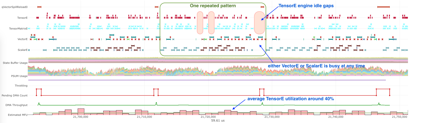
Fig. 59 A VectorE/ScalarE-bound profile.

Optimization: A common optimization to tackle vector/scalar-operation-heavy operators is combining instructions using low-level nki.isa APIs. Combining instructions can leverage the deep pipelined stages within VectorE and ScalarE engine data path to increase hardware utilization per instruction and reduce the instruction count. Check out the architecture guide to learn what operations can be done in a pipeline fashion in a single VectorE/ScalarE instruction.

For example, below pseudo-code showcase combining three instructions into a single one on ScalarE. impl 1 and impl 2 are functionally equivalent, but impl 2 is 3x faster in terms of latency by touching the input data only once and running all three operations (multiply, add, exp) in a pipeline.

# input: data (tile[128, 512]), scale (tile[128, 1]) , bias (tile[128, 1])

# impl 1:
scaled = nki.language.multiply(data, scale)
shifted = nki.language.add(scaled, bias)
exp = nki.language.exp(shifted)

# impl 2:
exp = nki.isa.activation(nki.language.exp, data,
                         bias, scale)

Check out nki.isa APIs to understand low-level ISA API semantics, limitations, engine mapping, and rough estimates of performance cost.

See Fused Mamba tutorial for a concrete example to combine matrix-vector multiplication and exponential evaluation in a single nisa.activation instruction. Similarly, in Fused Self Attention tutorial, we combine the subtraction of the maximum with exponential in a single nisa.activation instruction in the Softmax operator.

Opt #7: TensorE only: Leverage fast weight load

Symptom: Let’s consider a matrix multiplication between two matrices of shape [M, K] and [K, N], with one of the following conditions:

1. M is significantly smaller than 128, while N is much larger than 128, or

2. the other way around: N is significantly smaller than 128, while M is much larger than 128

In NKI, if the matrix with min(M, N) dimension is mapped to the stationary tensor (x input tensor in nl.matmul and nisa.nc_matmul) for the TensorE LoadStationary instruction (details see architecture guide ), we will typically end up under-utilizing TensorE more severely compared to mapping such matrix to the moving tensor.

In neuron-profile, programmers can identify also this inefficient case by inspecting the src access patterns for LoadStationary and MultiplyMoving instructions on TensorE. For example, the below screenshot indicates a stationary tensor with 1 element per partition and a moving tensor with 128 elements per partition:

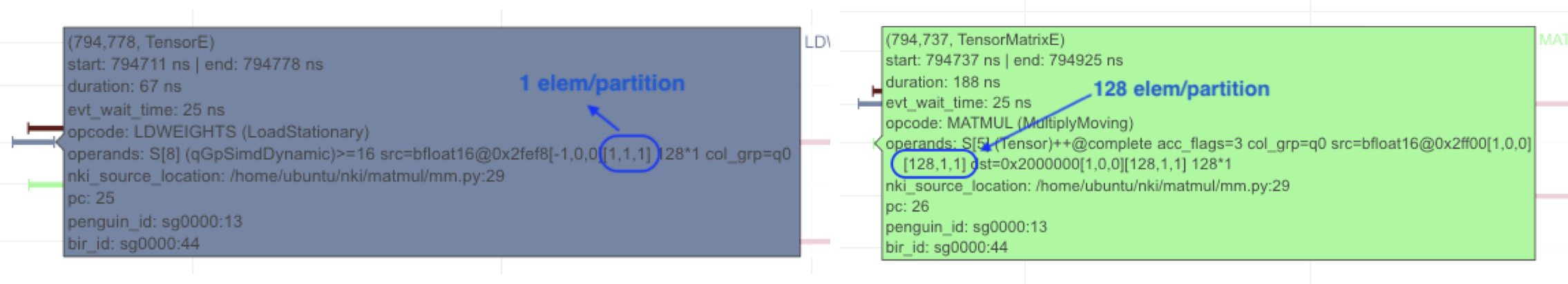
Fig. 60 Example instructions for matrix-vector multiplication.

If you have many back-to-back TensorE instructions with the above pattern, we recommend applying the below optimization.

Optimization: The key idea of this optimization is to simply swap the stationary and moving tensor positions for the given matmul in NKI, in order to leverage the “Fast LoadStationary” support in TensorE (more discussion in architecture guide). To better understand the intuition behind this, let’s walk through a concrete example.

Consider a [1, 128] x [128, 128] matrix multiplication as below:

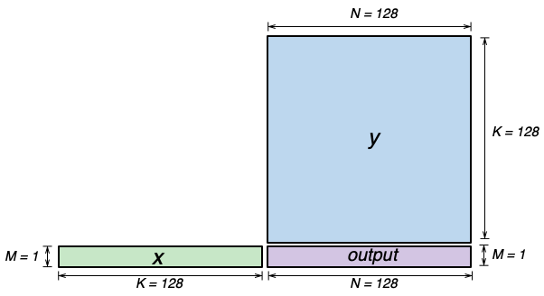
Fig. 61 Illustration of matrix-vector multiplication.

Since K=128 is the contraction dimension, it will get mapped to the partition dimension of the SBUF for both the x and y matrices. M and N will therefore get mapped to the free dimension of the SBUF. and we will refer to x as the “short” tensor, and y as the “long” tensor (short and long in the free dimension, respectively). We have two possible ways of performing this computation on the TensorE, which we’ll refer to as “Short Moving” and “Short Stationary“, depending on which tensor has the short free dimension.

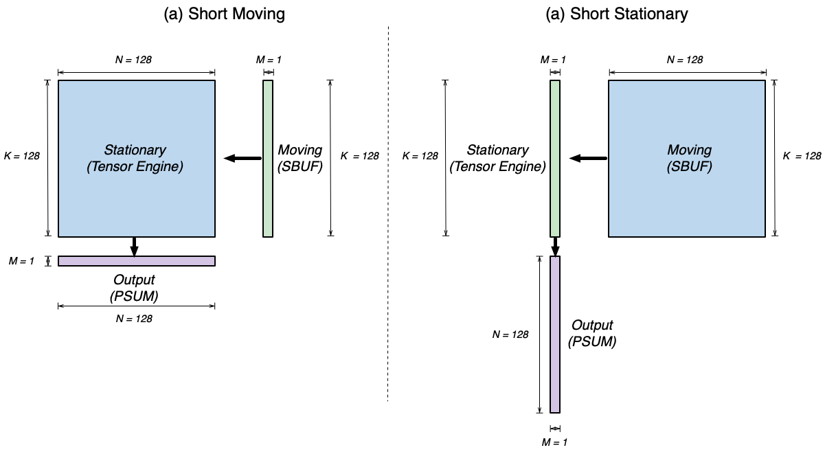
Fig. 62 Two possible TensorE instruction mapping for matrix-vector multiplication.

Based on the multiplication property of transpose, we have A×B=(B.T×A.T).T. Meanwhile, based on the semantics of TensorE, when we want to compute A×B, we need to call nc_matmul(A.T, B), and for BT×AT, we need to call nc_matmul(B.T.T, A.T) -> nc_matmul(B, A.T). Notice how the parameters to nc_matmul are swapped! Thus, when we swap stationary and moving tensors and perform the matrix multiplication, the output tensor will be transposed from the original output.

Recall, if there is a difference in initiation interval between LoadStationary and MultiplyMoving, one of them can end up limiting the throughput of TensorE:

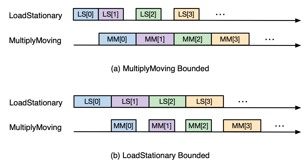
Fig. 63 Two possible TensorE performance characteristics.

In the above scenarios, we expect TensorE performance to be bound by whichever instruction reads the longer tensor - LoadStationary in “Short Moving”, and MultiplyMoving in “Short Stationary”. However, with TensorE Fast LoadStationary, TensorE can perform LoadStationary up to 4x faster than a MultiplyMoving with the same free axis size.

So in the two above scenarios:

1. Short Moving - LoadStationary initiation interval is roughly equal to the number of elements divided by 4 (because of fast LoadStationary), and MultiplyMoving initiation interval is dominated TensorE instruction turnaround time MM_INIT_LATENCY (64 cycles on trn1). Therefore, we have LS_II ~= 128/4 = 32 cycles , and MM_II ~= max(1, MM_INIT_LATENCY=64 cycles) which leads to issuing a MM roughly every 64 cycles.

2. Short Stationary - MultiplyMoving initiation interval will dominate, which leads to issuing a MM roughly every 128 cycles.

Because of the above, we will prefer to map short tensors to the moving tensor in MultiplyMoving instruction in TensorE.

A classic example is a matrix-vector product. This is commonly seen in auto-regressive token generation in LLMs, where most of the matmuls occur only on a single token (vector) as the feature map, while the weight tensor remains large and hence must be broken into tiles to meet TensorE tile size constraints.

Opt #8: TensorE only: Mitigating overhead from tensor transposes

Symptom: Since TensorE accounts for over 90% of the hardware FLOPS on a NeuronCore, we would like the engine to perform useful computations as much as possible, especially in matmul-heavy kernels. The most common “not useful” computation that could occupy precious TensorE cycles is tensor PF-transposes, which swap the partition and free dimensions of a NKI tile. When you have a profile with TensorE visually extremely busy, we recommend doing a sanity check on how much of the TensorE activities are performing transposes. One easy way to check is by selecting Instruction Type as the Instruction Grouping in View Settings :

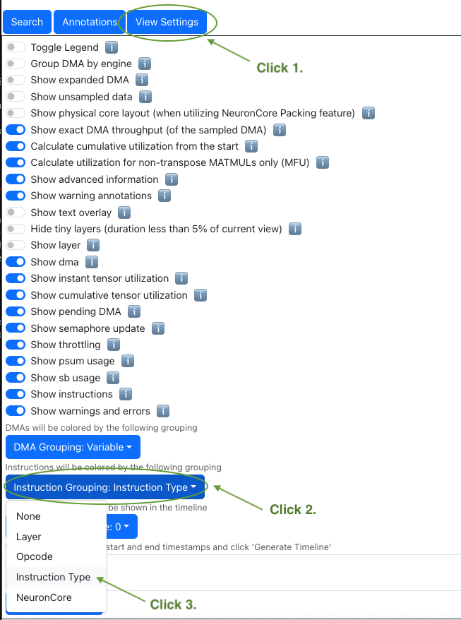
Fig. 64 Change view settings to visualize transposes.

With this instruction coloring, TensorE instructions will be highlighted in two different colors: one for Transpose and one for Regular (useful matmuls). As an example, the below profile has an execution trace with TensorE being the performance bottleneck. Visually, we can see the bulk of the TensorE execution is for regular matmuls, but there is a noticeable chunk of engine time spent on transpose-induced instructions in red. Note, the colors for transpose versus regular instructions are chosen randomly by the profiler each time. You should hover over the instructions to check the Instruction Type field on the pop-up to confirm the color mapping.

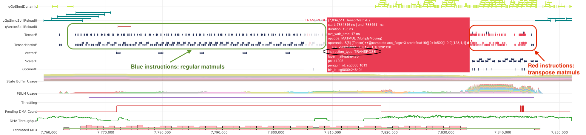
Fig. 65 Example timeline with a transpose instruction type.

Optimization: The key goal of this optimization is to reduce the number of transpose-induced instructions on TensorE, when such instructions are taking up a large portion of the execution. Before diving into techniques to reduce transposes, it is important to understand the root cause of these transposes.

At a high level, tensor transposes are needed to adjust the data layout of tensors to match the partition dimension requirements of different ISA instructions. Refer to the architecture guide for layout requirements of each compute engine. Transposes are inserted explicitly into NKI kernels through nl.transpose or nisa.sb_transpose APIs, or calling nl.matmul with transpose_x=False. These transposes are most commonly lowered down to Tensor Engine.

Broadly speaking, there are 2 different types of tensor transposes, with different root causes:

1. IO tensor transpose (abbreviated as IO transpose)

2. intermediate tensor transpose (abbreviated as intermediate transpose)

IO transpose. These transposes are ** done on NKI kernel IO (input/output) tensors, which must reside in device memory in current NKI releases. The transposes are needed when the NKI compute API consuming input tensors or producing the output tensors expect a different layout than their IO layout in device memory. To simplify discussion, we dive into input tensor layout discussion below, but the same reasoning also applies to output tensors.

For example, say we have an input tensor in device memory with layout [out_channel=128, in_channel=128] (major-to-minor ordering), but the nisa.nc_matmul call in our NKI kernel expects [in_channel, out_channel] as input tile layout. In this case, we can perform a nl.load to load the input into SBUF, with out_channel being the partition dimension because out_channel is the most major dimension in device memory. Then, a PF-transpose on TensorE is required before the loaded data can be consumed by nisa.nc_matmul . Alternatively, we can invoke nl.load_transpose2d to transpose the input tensor on the fly in the DMA engine, with a major caveat of much lower DMA bandwidth compared to nl.load. nl.load_transpose2d could make sense in a compute-bound kernel, but should certainly be avoided in memory-bound kernels.

Either way, an IO transpose is inevitable here due to the IO tensor layout choice we made as NKI programmers. In the naive case scenario where we only care about reaching the best performance for a single kernel, we can carefully decide on the IO tensor layout to make sure it is compatible with the NKI compute API layout requirements. When the input tensor is consumed by multiple compute APIs with conflicting layout requirements, IO-transposes cannot be avoided but should still be minimized as much as possible with a careful trade-off.

However, NKI kernels are often injected into a larger model defined at the framework such as PyTorch and JAX, in which case the kernel IO tensors are also input/output of the surrounding framework operators. These cases will require more complex reasoning on the optimal IO tensor layout for the NKI kernel, but the optimization goal of minimizing IO transposes remains the same.

One last complexity in deciding IO tensor layout is the layout choice also has a potential impact on DMA efficiency. See more discussion in a later section discussion optimizing data movement efficiency.

Intermediate Transpose. These transposes are done on intermediate tensors produced within a NKI kernel. These transposes arise due to layout requirement mismatches between producer and consumer NKI compute APIs.

There are two common techniques to reduce intermediate transposes: 1) swapping moving/stationary tensors in nisa.nc_matmul (or equivalently, nl.matmul) and 2) mapping a computation to an alternative engine with different layout requirements.

One example for technique 1) is in an operator chain commonly seen in Transformer models: linear_layer → layernorm. Normally, we tend to map the weight [hidden_size, 4xhidden_size] tensor in linear_layer to the stationary tensor and the input feature map [hidden_size, seq_len] to the moving tensor when performing nisa.nc_matmul on TensorE. The output feature map of this matmul will be in a layout of [4xhidden_size, seq_len]. However, the first step in layernorm to calculate mean and variance, nisa.bn_stats, requires 4xhidden_size to be the free dimension because we need to calculate mean/variance within a single token. Therefore, a naive implementation of this operator chain will trigger a PF-transpose between the nisa.nc_matmul and nisa.bn_stats instructions. However, if we were to instead map the weight tensor to the moving tensor and input feature map to stationary tensor, we can skip this PF-transpose entirely because the nisa.nc_matmul output will be in the expected layout by nisa.bn_stats.

An example for technique 2) is in a similar operator chain: linear_layer → RMSnorm with the same intermediate tensor dimensions as the above example. RMSnorm is considered a cheaper normalization operator compared compared Layernorm, because it replaces the mean/variance calculation with squared and summation. Unlike nisa.bn_stats for mean/variance calculations which must be done along the free dimension, for RMSnorm the scalar squared operator has no layout requirement and the summation can be done along either dimensions: use VectorE nisa.tensor_reduce for free dimension summation or use TensorE nisa.nc_matmul for partition dimension summation (see TensorE alternative use case in the architecture guide). Since RMSnorm can be done with either [4xhidden_size, seq_len] or [seq_len, 4xhidden_size], we should make the layout choice based on more surrounding operator: RMSnorm in Transformer models is typically followed by yet another linear_layer, which requires the [4xhidden_size, seq_len] layout. Therefore, to minimize intermediate transposes in an operator chain like linear_layer → RMSnorm → linear_layer , we should map the weight tensor of the first linear_layer to the stationary tensor and leverage TensorE to perform cross-partition summation for RMSnorm.

Optimizing Data Movement Efficiency

The key goal of optimizing memory-bound kernels is to keep the DMA engines running at high bandwidth utilization as much as possible. If you are seeing major DMA engine idle gaps in neuron-profile, you should first find ways to hide compute behind DMA activities using techniques discussed in Opt #4. The rest of this section is going to focus on optimizations to improve DMA bandwidth utilization. All the optimizations below are applicable to a common symptom: computation blocked by DMA activities, which are keeping the DMA engines “busy” but at low bandwidth utilization (< 60%):

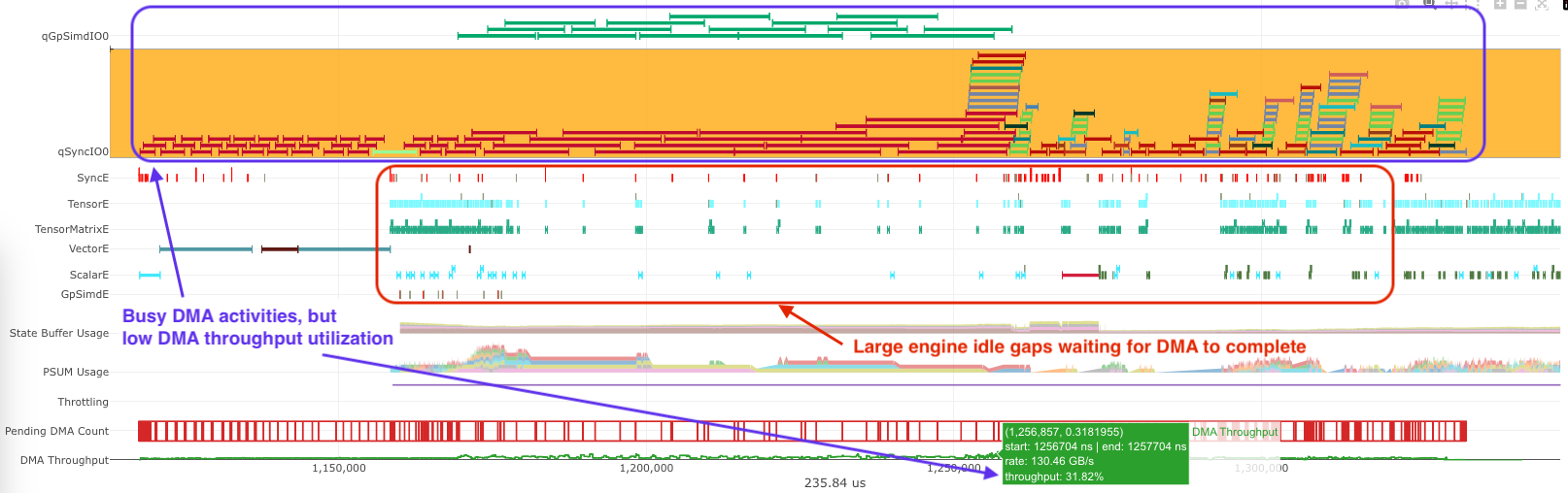
Fig. 66 Busy DMA engines with relatively idle compute engines.

Note, the current NKI release only supports running a kernel on a single NeuronCore (subject to changes in future releases). Therefore, the optimizations below will focus solely on movement between device memory and on-chip memory SBUF for now.

Opt #9: Perform sufficiently large DMA transfers

Symptoms: A quick way to determine whether the DMA transfers are moving large enough amount of data per transfer is to visualize the DMA activities per engine in neuron-profile:

Fig. 67 Change view settings to visualize DMA transfer per DMA engine.

With the above view settings, each DMA transfer will be shown with a continuous bar on the execution trace, grouped by DMA engines. Below is a profile example with small DMA transfers going on all 16 DMA engines. Visually, we can see DMA engine empty gaps (due to DMA overhead) are taking up more time than active DMA transfers. Hovering over some of DMA transfers, we can also see a transfer size of 4B, which is extremely tiny. For reference, the transfer size on Trainium/Inferential2 should be larger than 32KiB to achieve ideal bandwidth.

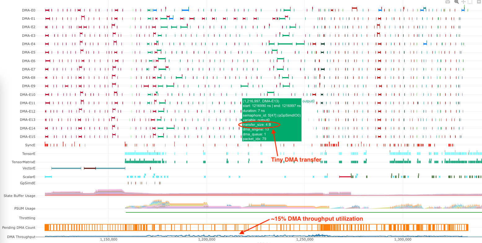
Fig. 68 Example timeline with tiny DMA transfers.

For comparison, here’s another profile with sufficiently large DMA transfers, achieving close 70% DMA throughput utilization:

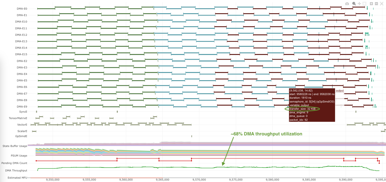
Fig. 69 Example timeline with large DMA transfers.

Optimizations: Refer to the architecture guide for more detailed discussion on DMA engines and intuitions behind the need for large DMA transfer sizes to achieve good DMA efficiency. Here, we will discuss simple rule of thumbs in NKI to trigger large DMA transfers: maximize the partition and free dimension sizes in both nl.load and nl.store. For example, the below data loading will trigger 16 DMA transfers that can be run on all 16 DMA engines, which each transfer loading 8 SBUF partitions’ worth of data with a transfer size of 32KiB:

import neuronxcc.nki.language as nl

def load_store_32kib_contiguous(in_tensor, out_tensor):
    # both in_tensor and out_tensor have FP32 data type, 4B/element
    assert in_tensor.dtype == out_tensor.dtype == nl.float32
    # both have shape 128x1024 in device memory
    assert in_tensor.shape == out_tensor.shape == [128, 1024]

    # partition dim size is at maximum supported by the architecture: 128
    # free dim size is at the ideal size to achieve good bandwidth usage: 1024
    # Beyond 1024 has diminished return on bandwidth and
    # runs the risk of degrading compute/data movement pipelining efficiency
    i_p, i_f = nl.mgrid[0:128, 0:1024]

    # This access pattern should map to 16 DMA transfers (1 transfer/DMA engine),
    # with each DMA transfer moving 8 partitions worth of data:
    # 8 partitions * 1024 elements * 4B/element = 32 KiB
    data_tile = nl.load(in_tensor[i_p, i_f])

    # Do some useful computation
    ...

    # Store, similar size as the load
    nl.store(out_tensor[i_p, i_f], data_tile)

Opt #10: Minimize use of DMA transposes.

Symptom: Excessive use of DMA transposes, invoked through nl.load_transpose2d, can degrade DMA bandwidth significantly. In neuron-profile, you can find out whether nl.load_transpose2d is taking up substantial amount of execution time by using the search functionality, which will highlight all the DMA activities that perform transposes on the fly:

Fig. 70 Search for DMA activities that perform transposes.

Optimizations: Refer to Opt #8 for a detailed discussion on how to eliminate the need of transposes on device memory input data. When the transposes are inevitable and the kernel is memory bound, we recommend replacing nl.load_transpose2d with nl.load() and nisa.nc_transpose(). For example, if you have an in_tensor of shape [8192, 128] in device memory but you would like an SBUF tile of shape [128, 8192] spread across 128 partitions for computation, the following two code snippets can achieve the same functionalities:

# Option 1, low DMA bandwidth usage:
sbuf_opt1 = nl.load_transpose2d(in_tensor[0:8192, 0:128])

# Option 2, better DMA bandwidth usage, fastest transpose:
sbuf_opt2 = nl.ndarray((128, 8192), dtype=in_tensor.dtype)
for i_in_tile in nl.affine_range(8192 // 128):
    i_start = i_in_tile*128
    current_tile = nl.load(in_tensor[i_start:i_start+128, 0:128])
    sbuf_opt2[0:128, i_start:i_start+128] = nisa.nc_transpose(current_tile)

Option 2 above is especially great for cases where nl.load_transpose2d is slowing down data movement in the critical path and TensorE is otherwise idle. Occasionally Option 1 can still be the right call, when the amount of data to be transposed is small and the overhead of nl.load_transpose2d can be well hidden behind other useful computation.

This document is relevant for: Inf2, Trn1, Trn1n