This document is relevant for: Inf1, Inf2, Trn1, Trn2, Trn3
Neuron Batching#
Batching refers to the process of grouping multiple samples together, and processing them as a group (i.e. passing them together through the neural network). Batching is typically used as an optimization for improving throughput at the expense of higher latency (and potentially higher memory footprint). Batching considerations are slightly different between inference and training workloads, and we thus cover them separately below.
Batching in inference workloads#
What is batched inference?#
The concept of batched inference is conceptually illustrated below, with a single NeuronCore performing batched computation of a 3 layer neural network with a batch-size of 4. The NeuronCore reads the parameters for a certain layer from the external memory, and then performs the corresponding computations for all 4 inference-requests, before reading the next set of parameters (thus, performing more compute for every parameter read from memory).

What are the benefits of batched Inference?#
For inference, batching is typically used as a trade-off knob between throughput and latency: higher batch-size typically leads to better hardware utilization and thus higher throughput, but at the same time batching requires to perform more computation until getting the first results, and hence leads to higher latency.

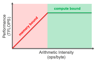
To understand why batching tends to improve throughput (up to a certain max value), it is useful to consider an intuitive visual performance-model called ‘the roofline model’, which provides with a theoretical bound on the system’s performance:

The X-axis indicates the arithmetic intensity (AI) of the workload, which is the ratio between the number of operations and the number of bytes read-from/written-to memory. The Y-axis indicates the theoretical extractable performance. For small(large) AI values, the workload is expected to be memory(compute) bound. For inference workloads, AI is often approximated by dividing the model’s number of operations by its memory footprint (#params x dtype_size). To a first order approximate, the AI value is linearly dependent on the batch-size, which means that the workloads performance (throughput) is expected to increase with the batch-size. To understand this more intuitively, for a larger batch size, Neuron can better amortize the cost of reading parameters from the external memory, and thus improve the overall hardware efficiency. It should be noted that while the roofline model can be very useful, it is not perfectly accurate (e.g. it doesn’t take into account spill/fills from/to on-chip SRAM memories), and thus users are encouraged to use it as a tool for estimating the optimal batch-size for their workloads.
How to determine the optimal batch-size for inference workloads?#
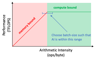
The optimal batch size is dependent on the application-level requirements: some applications require strict latency guarantees (in which case, check out the NeuronCore Pipeline technology), while other applications strictly aim to maximize throughput. We thus encourage our users to try out multiple batch-sizes, and compare performance between them. A good starting for batch-size exploration can be identified using the roofline model: we can choose a batch-size that achieves an Arithmetic Intensity which is at the edge of the compute bound region. By doing that, we aim to achieve max throughput with a minimal batch-size, and thus minimal impact to latency.

This can be expressed via the following
equation:
batch-size(Inference) = ceiling[0.5 x (<NeuronDevice PeakFLOPS>/<NeuronDevice MemBW>) /
(<model FLOPs>/(<#model-dense-params> x <dtype_size>))] (for
NeuronDevice PeakFLOPS and MemBW, see the Trainium Architecture, Inferentia Architecture and Inferentia2 Architecture pages.
For example, a BF16 BERT-Large model, with a sequence length of 128, will have the following approximated batch sizes:
Model |
NeuronDevice |
Peak TFLOPS (BF16) |
MemBW (GB/sec) |
Model GFLOPs |
Model Dense Params (Millions) |
Data-type size (BF16) |
Approximated optimal batch-size |
|---|---|---|---|---|---|---|---|
BERT-Large (SeqLen=128) |
Inferentia |
64 |
50 |
77.3 |
302 |
2 |
6 |
BERT-Large (SeqLen=128) |
Trainium |
210 |
820 |
77.3 |
302 |
2 |
2 |
ResNet-50 |
Inferentia |
64 |
50 |
7.8 |
25 |
2 |
5 |
ResNet-50 |
Trainium |
210 |
820 |
7.8 |
25 |
2 |
1 |
We recommend to evaluate multiple batch sizes and compare the performance between them, in order to determine the optimal latency/throughput deployment-point.
How to set the batch-size?#
The Neuron compiler takes a model and its sample input, as inputs for the compilation process. For example, the code snippet below will compile a model with a batch-size of 4:
import torch
import torch_neuron
from torchvision import models

# Load the model and set it to evaluation mode
model = models.resnet50(pretrained=True)
model.eval()

# Compile with an example input of batch size 4
image = torch.rand([4, 3, 224, 224])

model_neuron = torch.neuron.trace(model, image, dynamic_batch_size=True)

# Execute with a batch of 12 images
batch = torch.rand([12, 3, 224, 224])
results = model_neuron(batch)
For ahead-of-time compiled inference graphs (i.e. Inf1), dynamic batching can be used (as shown in the above code snippet) to process a larger client-side inference batch-size, and allow the framework to automatically break up the user-batch (12 in our case) into smaller batch sizes, to match the compiled batch-size (4 in our case). This technique increases the achievable throughput by hiding the framework-to-neuron overhead, and amortizing it over a larger batch size.
See also
Dynamic Batching in
torch-neuronxSpecial Flags in
tensorflow-neuronx.
Batching in training workloads#
Unlike inference workloads, training is inherently an offline process, and thus doesn’t have latency requirements. This means that training is almost always batched to some degree.
Batch-size naming#
For distributed processing, defining the batch size depends on the observation level. There are multiple terms you should be aware of when running a distributed training job, especially global batch size (GBS) and micro-batch. Knowing the batch size in advance is crucial for precompiling the computational graph and for setting the hyperparameters.
- micro-batch size
Smallest unit of the number of samples getting processed in a single step in the accelerator. For very large models, it is frequently chosen to be 1.
- gradient accumulation
Process of iterating over a micro-batch multiple times and summing up the gradients before an optimizer update. This can happen in a dedicated loop for gradient accumulation or as part of multiple iterations of samples in pipeline parallelism. See Developer guide for Pipeline Parallelism for more details on pipeline parallelism.
- data-parallel size (or DP degree)
Number of model replicas that process different portions of data in parallel. Each replica maintains a complete copy of the model while processing unique data chunks, after which their gradients are synchronized for the optimizer update. See Neuron Glossary for more details.
- global batch-size
Number of total samples used for an update of the optimizer. This includes all the respective gradients that get added up from data-parallel processing or gradient accumulation.
global batch size = micro_batch_size * data_parallel_size * gradient_accumulation_steps- mini-batch or replica-batch size
Number of samples that contribute to a gradient within one data-parallel rank. A mini-batch gradient is obtained by aggregating multiple micro-batch gradients within or without a pipeline (aka. gradient accumulation).
mini_batch_size = micro_batch_size * gradient_accumulation_steps- worker batch
The portion of mini-batch samples processed by a worker. The idea behind a worker batch is that one worker (node) might have a subset of the dp-degrees and we care about how much data gets tackled by this worker.
How to determine the optimal batch-size for training workloads?#
Determining the optimal batch-size for training workloads can be a non-trivial task. In most cases, we’d want to choose the largest batch-size that we can get away with.
The most dominant factor for determining the optimal batch-size in training workloads is memory footprint: training workloads have higher memory footprint compared to inference, as they require saving more tensors aside from the model parameters, such as gradients, intermediate activations (passed between forward-pass and backward-pass), and optimizer-state. If the batch-size is increased beyond a certain point, one can run out of device memory (indicated by an ‘Out of device memory’ error, typically abbreviated as OOM).
To estimate the memory footprint of a model, we look at the different contributors:
Weights and gradients:
typically 2B each, thus 4B per parameter
Optimizer state:
typically 4B - 12B per parameter
Intermediate activations:
sum of all tensor sizes for forward pass
for example, for a transformer neural network, this is roughly 16 x x <num_layers> x x x = 100MB x
For training workloads, determining the optimal batch size can be a little more tricky, due to two reasons:
Higher memory footprint: Training workloads have higher memory footprint compared to inference, as they require saving more tensors aside from the model parameters, such as gradients, intermediate-state and optimizer-state. If the batch-size is increased too much, one can run out of device memory (indicated by an ‘Out of memory’ error, typically abbreviated as OOM).
Arithmetic intensity estimation: Arithmetic intensity is harder to estimate in training workloads, compared to inference workloads, as the majority of the external memory access are due to reads/writes of intermediate activation state (rather than parameters), which requires lower level familiarity with the model to estimate correctly.
A good first order approximate for the optimal batch-size in a training
workload, is the largest one that can fit in the device’s memory (i.e.
won’t lead to OOM error).
batch-size(Training) = 0.6 x (<TP-Rank> x <PP-Rank> x ``<NeuronCore MemoryCapacity>)
/ ``(<#model-dense-params> x ``<model-state-bytes-per-parameter>)
Note TP-rank stands for Tensor-Parallelism rank, i.e. how many NeuronCores participate in a single Tensor-Parallelism group. Similarly, PP-rank stands for Pipeline-Parallelism rank, i.e. how many NeuronCores participate in a single Pipeline-Parallelism group.
For example, for BERT-Large Ph1 training, with a model-state of 4B per
parameter (2B weights, 2B parameters), and TP-rank = PP-rank = 1, the
approximated optimal per-NeuronCore training batch-size would be:
batch-size(Training/Trainium) = 0.6 x (1 x 1 x 16e+9`) / (300e+6 x 4) = 8`
This document is relevant for: Inf1, Inf2, Trn1, Trn2, Trn3
