Profiling PyTorch Neuron (torch-neuronx) with TensorBoard
Contents
This document is relevant for: Inf1, Inf2, Trn1, Trn1n
Profiling PyTorch Neuron (torch-neuronx) with TensorBoard#
Table of Contents
Introduction#
Neuron provides a plugin for TensorBoard that allows users to measure and visualize performance on a torch runtime level or an operator level. With this information, it becomes quicker to identify any performance bottleneck allowing for quicker addressing of that issue.
For more information on the Neuron plugin for TensorBoard, see Neuron Plugin for TensorBoard (Trn1).
Setup#
Prerequisites#
Initial Trn1 setup for PyTorch (torch-neuronx) has been done
Environment#
#activate python virtual environment and install tensorboard_plugin_neuron
source ~/aws_neuron_venv_pytorch_p38/bin/activate
pip install tensorboard_plugin_neuronx

#create work directory for the Neuron Profiling tutorials
mkdir -p ~/neuron_profiling_tensorboard_examples
cd ~/neuron_profiling_tensorboard_examples
Understanding the Operator Level Trace#
Goal#
After completing this tutorial, the user should be able to understand the features of the Operator Level Trace. The user should also be able to form a narrative/surface level analysis from what is being presented in the Operator Level Trace.
Set Up#
Let’s set up a directory containing the material for this demo
cd ~/neuron_profiling_tensorboard_examples
mkdir tutorial_1
cd tutorial_1

# this is where our code will be written
touch run.py
Here is the code for run.py:
import os
import torch
import torch_neuronx
from torch_neuronx.experimental import profiler
import torch_xla.core.xla_model as xm

os.environ["NEURON_CC_FLAGS"] = "--cache_dir=./compiler_cache"

device = xm.xla_device()

class NN(torch.nn.Module):
   def __init__(self):
      super().__init__()

      self.layer1 = torch.nn.Linear(4,4)
      self.nl1 = torch.nn.ReLU()
      self.layer2 = torch.nn.Linear(4,2)
      self.nl2 = torch.nn.Tanh()

   def forward(self, x):
      x = self.nl1(self.layer1(x))
      return self.nl2(self.layer2(x))

with torch.no_grad():

   model = NN()

   inp = torch.rand(4,4)
   output = model(inp)

   with torch_neuronx.experimental.profiler.profile(
      port=9012,
      profile_type='operator',
      ms_duration=10000 ):


      # IMPORTANT: the model has to be transferred to XLA within
      # the context manager, otherwise profiling won't work
      neuron_model = model.to(device)
      neuron_inp = inp.to(device)

      output_neuron = neuron_model(neuron_inp)
      xm.mark_step()

print("==CPU OUTPUT==")
print(output)
print()
print("==TRN1 OUTPUT==")
print(output_neuron)
Understanding the Code#
For this first tutorial, we’ll be using a simple Feed forward NN model. However, once the TensorBoard dashboard is up, we’ll see some interesting and unexpected things. A simple model is helpful since it is easy to reference back to.
Another important part is the “operator” profiling type we specified in the context manager.
Low Level: The “operator“ dashboard is the dashboard that contains the Operator Level Trace This view also only zooms in on the NeuronDevice, while the ”trace“ dashboard shows processes from all devices. The Operator Level Trace View is organized by levels of abstraction, with the top level showing the model class. The next lower tier shows model components, and the lowest tier shows specific operators that occur for a specific model component. This view is useful for identifying model bottlenecks at the operator level.
We also print out the outputs from the CPU model and the TRN1 model to note the small differences in output.
Running The Profiler#
python run.py
Output:
Initial Output & Compilation Success
2022-10-12 19:02:02.176770: E tensorflow/core/framework/op_kernel.cc:1676] OpKernel ('op: "TPURoundRobin" device_type: "CPU"') for unknown op: TPURoundRobin
2022-10-12 19:02:02.177579: E tensorflow/core/framework/op_kernel.cc:1676] OpKernel ('op: "TpuHandleToProtoKey" device_type: "CPU"') for unknown op: TpuHandleToProtoKey
torch_neuron: The environment variable 'XLA_IR_DEBUG' is not set! Set this to '1' before your model is compiled to include model information for profiling! Environment variable will be set (and cleared) in this profile scope
torch_neuron: The environment variable 'XLA_HLO_DEBUG' is not set! Set this to '1' before your model is compiled to include model information for profiling! Environment variable will be set (and cleared) in this profile scope
Starting to trace for 10000 ms. Remaining attempt(s): 2
2022-10-12 19:02:02.259487: W tensorflow/core/profiler/lib/profiler_session.cc:105] Profiling is late by 402863 nanoseconds and will start immediately.
2022-10-12 19:02:02.259528: W tensorflow/libtpu/profile_manager.cc:310] ProfileManager::start: Environment variable NEURON_PROFILE not set - not enabling Neuron device profiling
2022-10-12 19:02:02.259541: W tensorflow/libtpu/profile_manager.cc:316] ProfileManager::start: Environment variable NEURON_PROFILE_TYPE not set - not enabling Neuron device profiling
2022-10-12 19:02:02.000325: INFO ||NCC_WRAPPER||: No candidate found under compiler_cache/neuron-compile-cache/USER_neuroncc-2.0.0.4226a0+8bf37708b/MODULE_5452102422278823855.
2022-10-12 19:02:02.000325: INFO ||NCC_WRAPPER||: Cache dir for the neff: compiler_cache/neuron-compile-cache/USER_neuroncc-2.0.0.4226a0+8bf37708b/MODULE_5452102422278823855/MODULE_0_SyncTensorsGraph.53_5452102422278823855_ip-172-31-33-242-2131b830-24512-5eadb072703d9/b6c38ec4-f890-4ab9-97e2-e6b7d2d78f65
.
Compiler status PASS
2022-10-12 19:02:05.000196: INFO ||NCC_WRAPPER||: Exiting with a successfully compiled graph
Note
The warnings about the XLA_IR_DEBUG and XLA_HLO_DEBUG
env vars not being set can be ignored for the most part. This warning
only comes into play when compiling the model for Neuron outside of the
profiler context manager.
Processing the Neuron Profiler Traces
torch_neuron: Waiting for xplane files ...
torch_neuron: Decoding xplane files from profiler
torch_neuron: translate_xplane: Processing plane: '/host:CPU'
torch_neuron: XLA decode - Read filename 2022_10_26_18_00_39
torch_neuron: XLA decode - Read date parts ['2022', '10', '26', '18', '00', '39']
torch_neuron: XLA decode - Read start date 2022-10-26 18:00:39 from directory stamp
torch_neuron: translate_xplane: Processing plane: '/host:Neuron-runtime:profile//822ac0425c2b4163_1/model10001/node5/plugins/neuron/1666807250/neuron_op_timeline_split.json'
torch_neuron: translate_xplane: Writing plane: '/host:Neuron-runtime:profile//822ac0425c2b4163_1/model10001/node5/plugins/neuron/1666807250/neuron_op_timeline_split.json' to 'temp_profiler_logs/822ac0425c2b4163_1/neuron_op_timeline_split.json'
torch_neuron: translate_xplane: Processing plane: '/host:Neuron-runtime:profile//822ac0425c2b4163_1/model10001/node5/plugins/neuron/1666807250/neuron_op_timeline.json'
torch_neuron: translate_xplane: Writing plane: '/host:Neuron-runtime:profile//822ac0425c2b4163_1/model10001/node5/plugins/neuron/1666807250/neuron_op_timeline.json' to 'temp_profiler_logs/822ac0425c2b4163_1/neuron_op_timeline.json'
torch_neuron: translate_xplane: Processing plane: '/host:Neuron-runtime:profile//822ac0425c2b4163_1/model10001/node5/plugins/neuron/1666807250/neuron_framework_op.json'
torch_neuron: translate_xplane: Writing plane: '/host:Neuron-runtime:profile//822ac0425c2b4163_1/model10001/node5/plugins/neuron/1666807250/neuron_framework_op.json' to 'temp_profiler_logs/822ac0425c2b4163_1/neuron_framework_op.json'
torch_neuron: translate_xplane: Processing plane: '/host:Neuron-runtime:profile//822ac0425c2b4163_1/model10001/node5/plugins/neuron/1666807250/neuron_hlo_op.json'
torch_neuron: translate_xplane: Writing plane: '/host:Neuron-runtime:profile//822ac0425c2b4163_1/model10001/node5/plugins/neuron/1666807250/neuron_hlo_op.json' to 'temp_profiler_logs/822ac0425c2b4163_1/neuron_hlo_op.json'
torch_neuron: Trace file: temp_profiler_logs/neuron_trace.json
torch_neuron: Translated JSON files: ['temp_profiler_logs/822ac0425c2b4163_1/neuron_op_timeline_split.json', 'temp_profiler_logs/822ac0425c2b4163_1/neuron_op_timeline.json', 'temp_profiler_logs/822ac0425c2b4163_1/neuron_framework_op.json', 'temp_profiler_logs/822ac0425c2b4163_1/neuron_hlo_op.json']
torch_neuron: Output processed JSON profiles
torch_neuron: Cleaning up temporary files
Printing output from CPU model and Trn1 Model:
==CPU OUTPUT==
tensor([[-0.1396, -0.3266],
        [-0.0327, -0.3105],
        [-0.0073, -0.3268],
        [-0.1683, -0.3230]])

==TRN1 OUTPUT==
tensor([[-0.1396, -0.3266],
        [-0.0328, -0.3106],
        [-0.0067, -0.3270],
        [-0.1684, -0.3229]], device='xla:1')
Loading the Operators Level Trace in TensorBoard#
Run tensorboard --load_fast=false --logdir logs/
Take note of the port (usually 6006) and enter localhost:<port> into
the local browser (assuming port forwarding is set up properly)
Note
Check Viewing the Trace on TensorBoard to understand TensorBoard interface
The Operator Level Trace views are the same format plus an id at the
end; year_month_day_hour_minute_second_millisecond_id. The Tool
dropdown will have 3 options: operator-framework, operator-hlo, and
operator-timeline.
Operator Framework View#
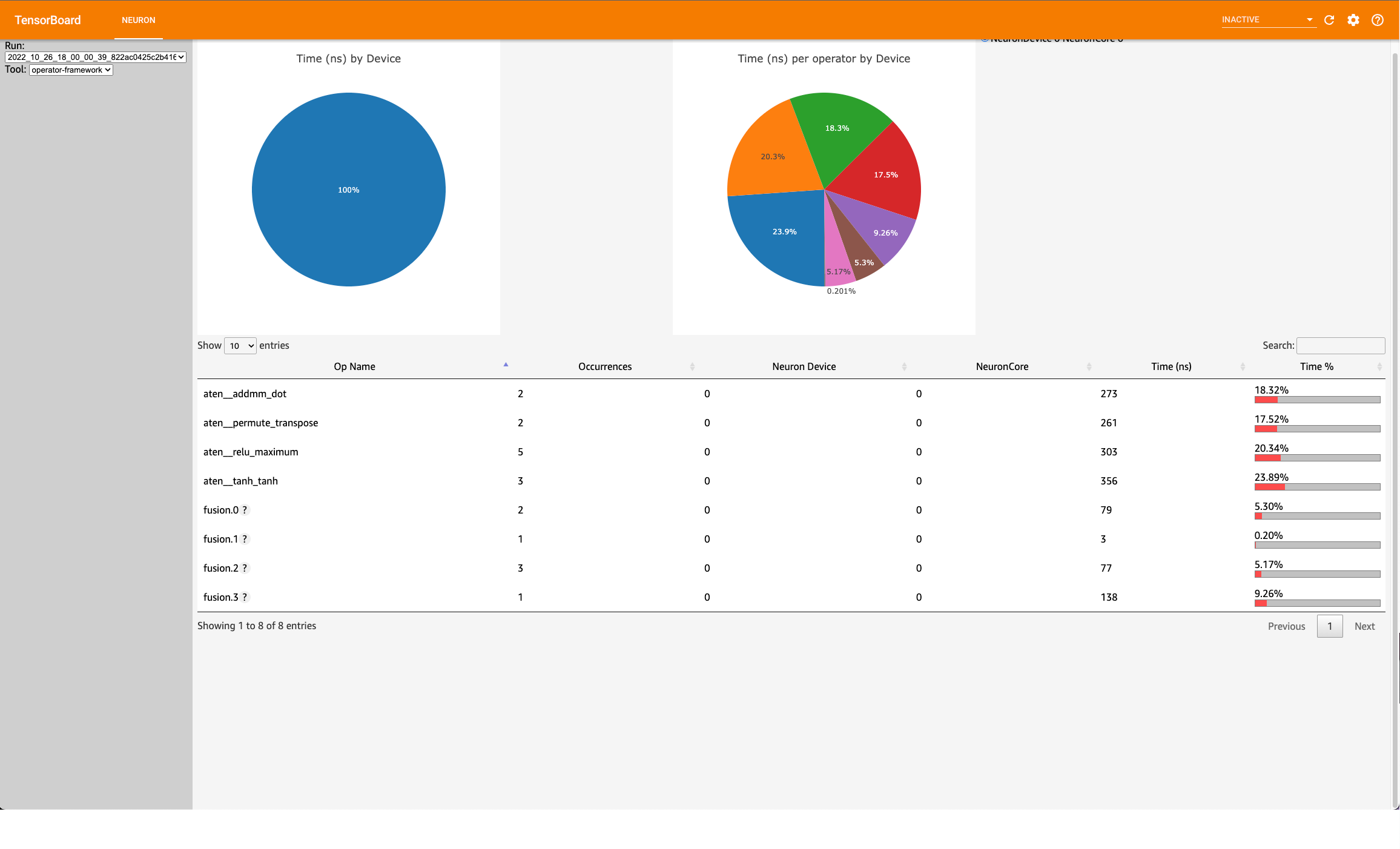
This view contains a pie-chart displaying the proportional execution time for each of the model operators on the framework level for a neuron device. The list of operators is shown in the bottom along with other details about number of occurrences, execution time and neuron device and core.
Operator HLO View#
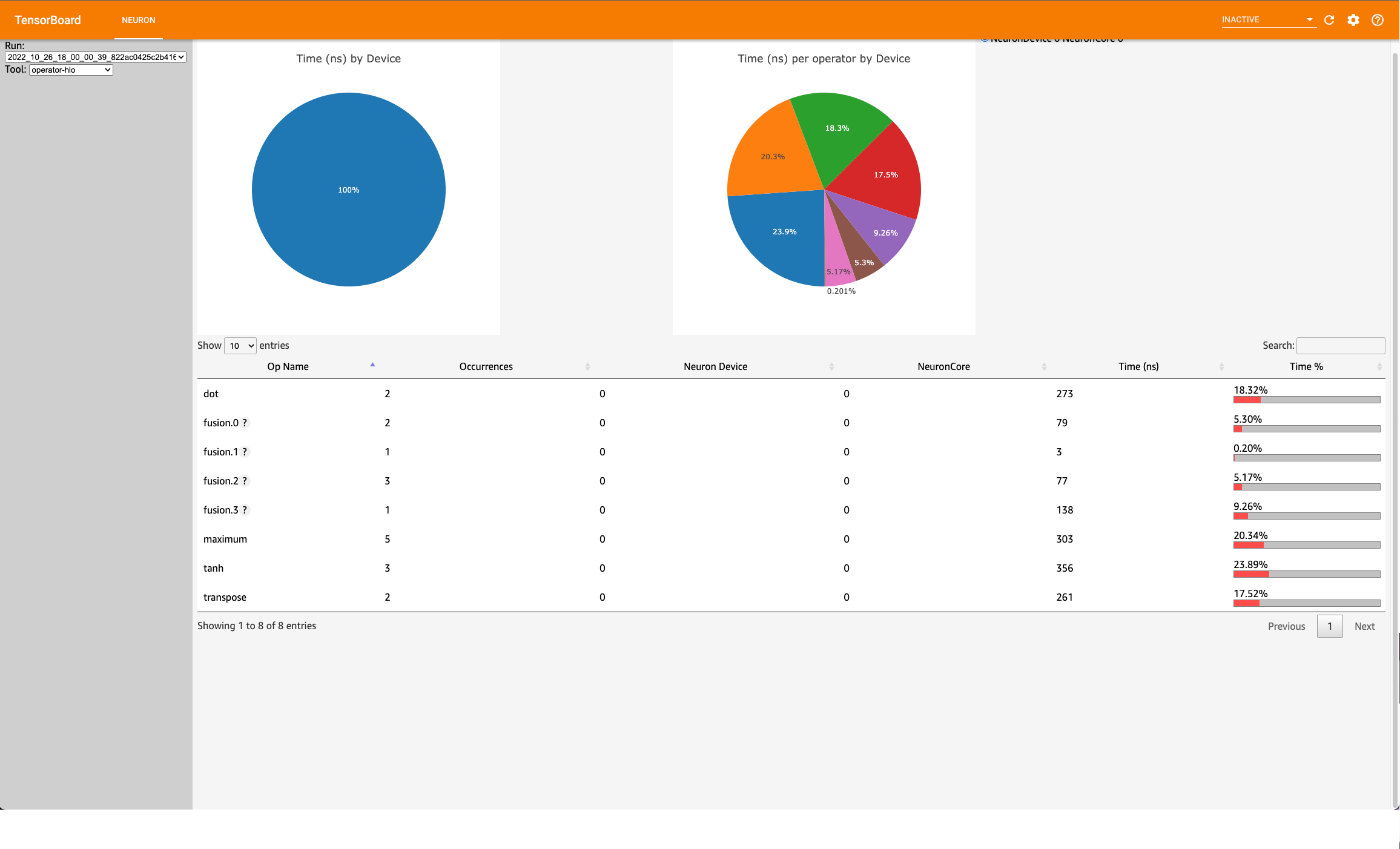
This view contains a pie-chart displaying the proportional execution time for each of the model operators on the hlo level for a neuron device. The list of operators is shown in the bottom along with other details about number of occurrences, execution time and neuron device and core.
Note
For this simple model, the pie chart will be the same as the framework view. This won’t be the case for larger and more complex models.
Operator Trace View#
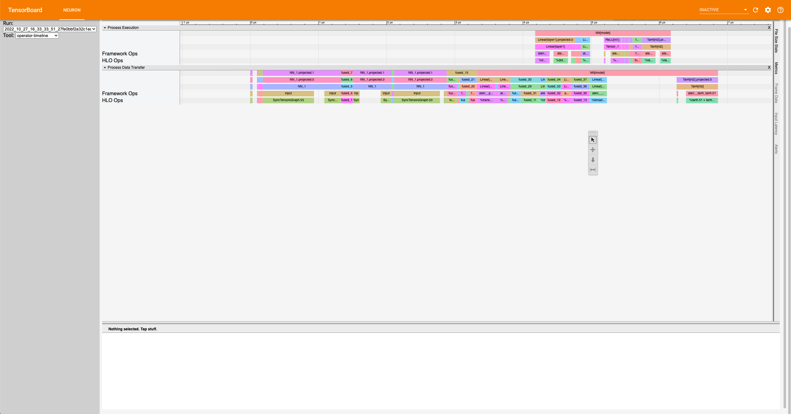
Execution vs. Data Transfer#
Notice there are two sections: Process Execution and Process Data Transfer. In each section there are more subdivisions with each layer representing a certain level of abstraction. Also important to note that the timescale axis is aligned between the two sections. This is important to note as sometimes there are gaps in the process execution. Most of the time, there are data transfer operations happening in between the gaps.
Fusion Operators#
Simple Case: Zooming in on the operations, we can recognize some operations for a neural network, such as a dot product and transpose, but sometimes there will be fused operators (fusion operators). To understand these operators, click on it, and on the bottom of the dashboard, some information will appear.
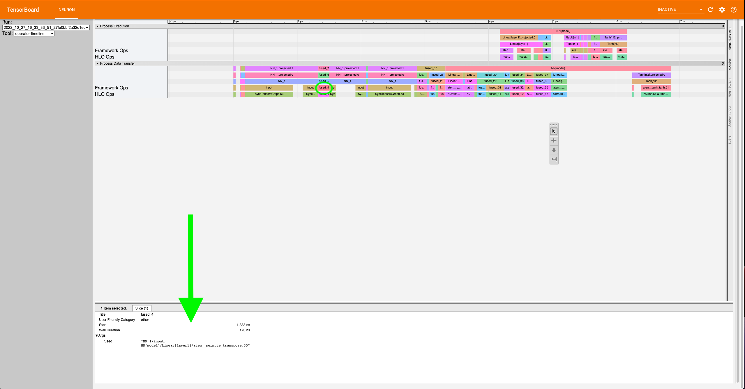
Notice in the above example the fusion operator is fusing the operator before and
after itself on the timeline. More specifically, fused_4 is a fusion
of NN_1/input and
NN[model]/Linear[layer1]/aten__permute_transpose.35. These kinds of
fusions occur when the neuronx-cc compiler has found an optimization
relating to the two operators. Most often this would be the execution of
the operators on separate compute engines or another form of parallelism.
Complex Case: Most often, the order of fusion operators can get a little complicated or contain “hidden” information. For the first example, let’s zoom into the data transfer section such that we see the timescale range from 3400 ns. to 5190 ns. It should look similar to below:
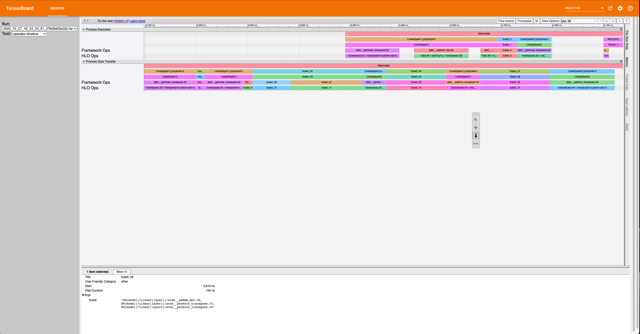
Looking at fused_28 (3819 ns.) we see it’s surrounded by other fused operators.
Furthermore, the fused_28 operator fuses more than two operators. NN[model]/Linear[layer1]/aten__addmm_dot.36,
NN[model]/Linear[layer1]/aten__permute_transpose.35, and NN[model]/Linear[layer2]/aten__permute_transpose.20.
Looking along the Framework Ops, we will find the transpose operators but not the aten__addmm_dot.36 operator. This can occur
because there is a complete overlap of operators. In other words, while there is a data load operation happening for
the transpose operators, a data load operation also occurs for the dot operator.
This also explains how fusion operators can be consecutive. From this, a couple of complexities arise regarding the “Start” time of these operators:
For operators completely hidden in the trace (except through fusion operators), the profiler won’t give a “Start” time. All that can be said is that it occurs sometime between the “Start” and “Start”+“Wall Duration” time length of the first fusion operator it is visible in (
fused_27(3782 ns.) for the dot operator). Similarly, the “Wall duration” can’t be determined exactly since the operator can extend across multiple fusion operators. For instance, looking atfused_31(3968 ns.) to the right offused_28, we see that specific dot operator for the last time.Just like operators would completely be hidden in a series of fusion operators, some operators might start or end singly. That is to say, they start or end without being parallel with other operators. This is visible when the trace block name is the operator itself. In these scenarios, the only way to accurately calculate the wall duration of a specific operator is if it starts singly and ends singly and has no fusion operators containing it before the start or after the end. If those conditions are met, then the wall duration can be calculated with exact precision. In all other scenarios the true wall duration cannot be accurately determined form the trace, but reasonable estimates can be formed.
Understanding the Low Level Timeline#
Looking at the trace we can look behind the scenes at how the model is executed on neuron hardware. Before proceeding with the analysis, it is worth recalling the way we defined the model for this tutorial:
class NN(torch.nn.Module):
   def __init__(self):
      super().__init__()

      self.layer1 = torch.nn.Linear(4,4)
      self.nl1 = torch.nn.ReLU()
      self.layer2 = torch.nn.Linear(4,2)
      self.nl2 = torch.nn.Tanh()

   def forward(self, x):
      x = self.nl1(self.layer1(x))
      return self.nl2(self.layer2(x))
Analysis#
ReLU at the beginning? The first couple of blocks in the Process Data Transfer section initially appear to be confusing. There is an Input (0 ns.)
block followed by a ReLU (100 ns.) operator. Under the hood here, ReLU is rewritten as an elementwise_max(arr,0),
(0 here means an array with zeros) but to create this operation, the zeros have to be set in memory, which is a data operation.
A general rule is that if an operator appears this early in the data transfer section, it most likely means there is an operation
lowering involving setting some values into memory for use later on.
Memory allocation for Linear[layer1]: We resume with the data transfer operations. Here, memory is getting allocated for specific operators, and sometimes the allocated
inputs get loaded onto operators while the rest of the input gets allocated. This can be seen at fused_4 (1333 ns.) and fused_8 (2078 ns.).
Eventually the input gets fully allocated, and other allocations occur for dot products, transpose, and broadcast operators for
Linear[layer1] and Linear[layer2].
Linear[layer2] transpose before ReLU on compute? Notice that as the Data Transfer Operations for Linear[layer2] start the computation (i.e Process Execution) for the Linear[layer1]
operators start. Analyzing the Process Execution trace for the Linear[layer1], we see an unusual ordering towards the end. We see a
transpose for Linear[layer2] occur before the ReLU activation function. This occurs because performing the transpose first would
optimize the calculation of the Linear[layer2] dot faster. Since ReLU must be calculated before the dot product, ReLU follows.
This is a quirk of the architecture of trn1.
Tanh before Linear[layer2] dot? The next step is the dot for Linear[layer2], but we notice that some Tanh operators appear before the dot operator. This can be
explained by the implementation of Tanh in the trn1 architecture/runtime. Simply put, Tanh utilizes a lookup table, and performs
interpolation on that table for error minimization. Pre-computation of the lookup table can occur before and during the dot operation.
We see this in the fused_12 (5611 ns.) operator. After the dot operator, the Tanh operator comes again, which would correspond to the
actual activation. We see some final data transfer operations, which have to do with output transfer from the Neuron device to host.
Conclusion#
There are a few conclusions that can be determined from analyzing the timeline. We can see that we’ve been able to save a bit of time due to
parallelism between computing Linear[layer1] and allocating memory for Linear[2] operations. There was also time saved with the parallelism
of Tanh and the dot operators for Linear[2]. Another clear trend is that a majority of the time (about 83%) is spent on data transfer operations.
It is also evident that even a simple Feed Forward NN becomes complicated when put under a microscope in the profiler. Facts such as the lowering
of ReLU to an elementwise_maximum and implementation of Tanh in the runtime/architecture, aren’t explicitly stated in the profiler, but do make
themselves known by the unusual ordering placement of the trace blocks.
In terms of action items that can be taken based on our narrative, there really isn’t any. This is a very very simple model that outputs after 6 microseconds, and we chose it because it is simple to understand. In more realistic examples we will aim to do more compute than data transfer on the hardware, and where possible to overlap data transfer and compute between sequential operations.
The profiler revealed a lot of optimizations that were done, via fusion operators and parallelism. However, the end goal of this tool is to be able to improve performance by revealing the bottlenecks of the model. In the next couple of tutorials, we will go over a more practical example where the profiler will reveal a bottleneck and we address it and visualize the improved performance using the trace and operator profile types.
Note
While we did explain some of the quirks visible in the profiler at a microscopic level, it isn’t necessary to do so for normal use. This tutorial introduced the microscopic explanation for these occurrences to show to the user that this is indeed what happens in the hardware when executing a simple FFNN.
This document is relevant for: Inf1, Inf2, Trn1, Trn1n