MXFP Matrix Multiplication with NKI on AWS Neuron#

In this guide, you’ll learn how to perform MXFP4/8 matrix multiplication, quantization, and Neuron’s recommended best practices for writing MX kernels.

Before You start#

Read the MX-related sections of the Trainium 3 Architecture Guide for NKI and become familiar with basic matrix multiplication concepts on Neuron in the Matrix Multiplication tutorial.

Note

The code snippets in this guide are taken from the tutorial code package which demonstrates how to execute all MX kernel examples from Torch. We recommend you browse and run the code as you read the tutorial.

What is MXFP4/8 Matrix Multiplication?#

MXFP4/8 matrix multiplication uses microscaling (MX) quantization as defined in the OCP standard. Unlike traditional quantization that uses tensor- or channel-wide scale factors, microscaling calculates quantization scales from small groups of values. Specifically, groups of 32 elements along the matrix multiplication contraction dimension share the same 8-bit MX scale value.

This approach preserves significantly more information in quantized values by preventing high-magnitude outliers from “squeezing” the entire data distribution. The NeuronCore-v4 Tensor Engine performs matrix multiplication of MXFP4 or MXFP8 input matrices and dequantization with MX scales in a single instruction, achieving 4x throughput compared to BF16/FP16 matrix multiplication while outputting results in FP32 or BF16.

Layout and Tile Size Requirements#

Before diving into code examples of MX multiplication, it’s important to review the layout and tile-size requirements of MX. MX quantized tensors are represented with separate data and scale tensors, each with distinct requirements.

Data Tensor#

Compared to BF16/FP32 matrix multiplication, the performance uplift from Matmul-MX comes from the ability to contract 4x more elements during one matmul operation as each TensorE processing element is able to perform four simultaneous, FP4/FP8, multiply-accumulate computations. This means the maximum effective contraction dimension has increased from 128 → 512.

First, let’s examine the tile-size constraints for MX so we can allocate the correct space for tensors. MX data is represented in NKI using quad (x4) packed data types (float8_e5m2_x4, float8_e4m3fn_x4, and float4_e2m1fn_x4, herein referred to collectively as MXFP_x4). The float8_*_x4 types are 32-bits wide and physically contain four float8 elements. The float4_*_x4 type is 16-bits wide and physically contains four float4 elements. As expressed in _x4 elements, the TensorE maximum tile sizes in NKI code continue to be given by the existing hardware constraints, summarized below.

Matrix Type	Data Type	Implied Physical Size	Max Tile Size in Code
Stationary	BF16	[128P, 128F]	[128P, 128F]
Stationary	MXFP_x4	[512P, 128F]	[128P, 128F]
Moving	BF16	[128P, 512F]	[128P, 512F]
Moving	MXFP_x4	[512P, 512F]	[128P, 512F]

This means that we will allocate data tensors, of type MXFP_x4, in our NKI code with the same shapes as we would for BF16/FP32, but it’s implied they contain 4x more contraction elements as shown in the subsequent diagrams.

Now let’s examine a BF16 tile destined to be quantized into a max-sized moving tile for Matmul-MX ([128P, 512F] MXFP_x4). Note that the following concepts are equally applicable to the stationary tile whose max size is [128P, 128F].

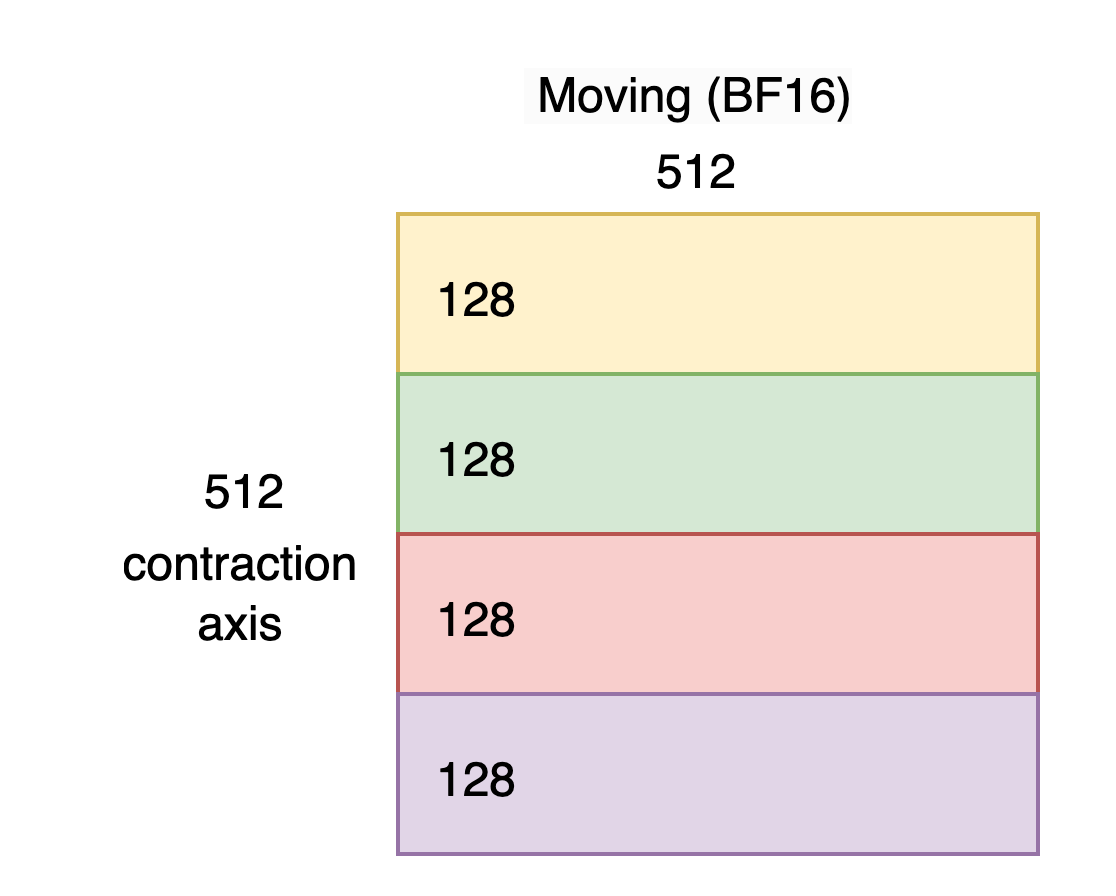
Since a 4x larger contraction dimension is supported we’ll start with a BF16 tile of size [512, 512] as shown below. To help us in the subsequent step we’ll also view it as being sectioned into 4 regions of 128 rows (i.e. reshaped as [4, 128, 512]). This view is mathematical (i.e. not residing in any particular memory).

As explained in the Trainium 3 Architecture Guide for NKI we must take 4 elements originating 128 apart on the contraction axis and pack them together on the SBUF free-dimension as shown below. We’ll call this transformation “interleaving”.

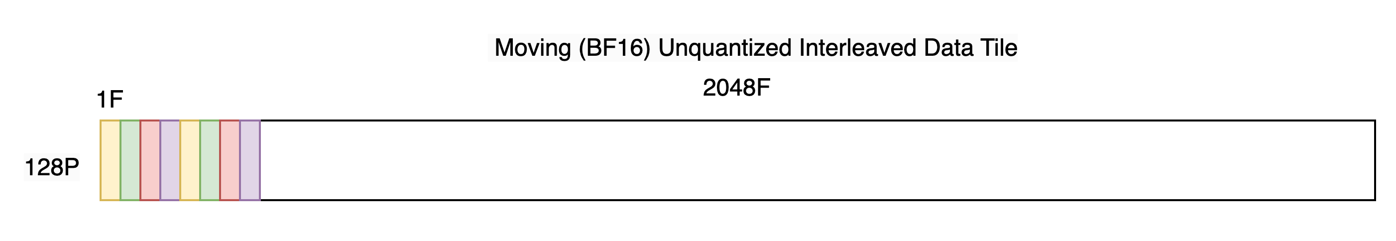
Notice the SBUF shape has become [128P, 2048F]. In a subsequent code example we’ll see that it’s useful to view/reshape this as [128P, 512F, 4F], making it clear we have 512 groups of 4 packed elements.

Next, let’s Quantize-MX this tile, which will preserve the layout but pack groups of 4 free-dimension elements into a single MXFP_x4 element, as shown below. Note that Quantize-MX does not support an FP4 output but Matmul-MX does support FP4 input.

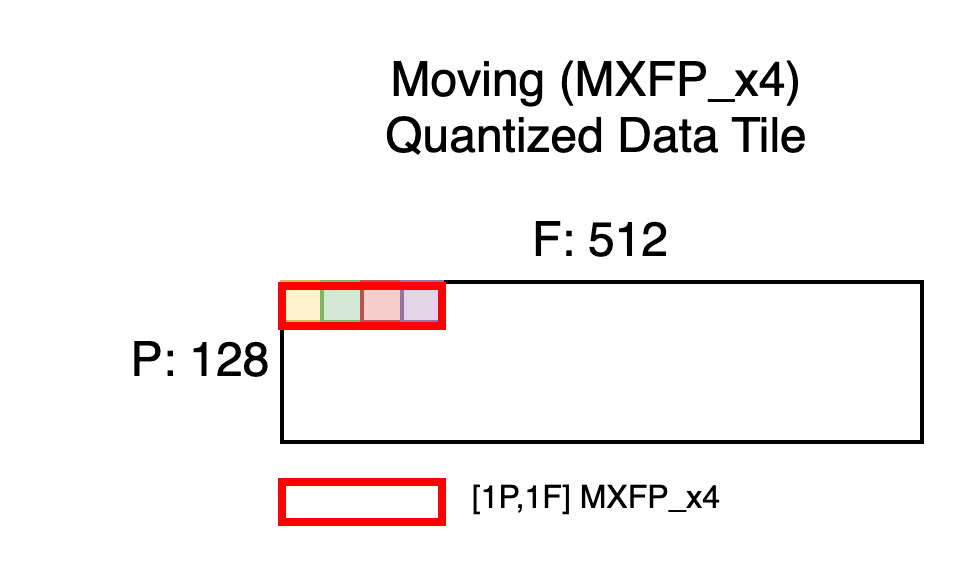
Notice the shape is now [128P, 512F] which is the max moving tile size we aimed for. But each MXFP_x4 element, shown in red, physically contains four quantized elements from the original tile. Recall that each TensorE processing element ingests enough data to perform four, FP4/FP8 multiply-accumulate operations, which is why four elements from the original contraction axis must be packed together in this fashion.

With this understanding we’ll state the space allocation rules for quantized MXFP_x4 data tiles.

Unquantized Interleaved Data Tile = [P,F] BF16 in SBUF

MX Quantized Data Tile = [P, F//4] MXFP_x4 in SBUF

Scale Tensor#

Let’s revisit the BF16 tile with the interleaved SBUF layout but this time with one of the [8P, 4F] scaling groups overlaid.

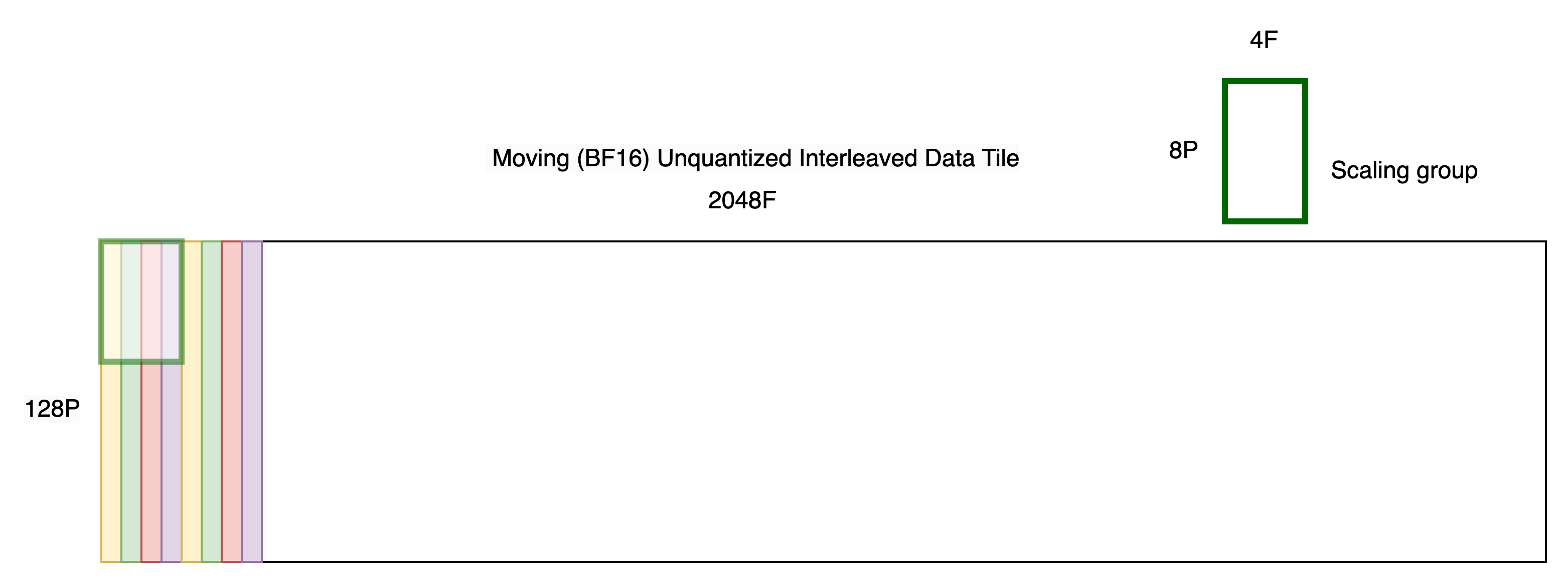
MX scales are represented using a UINT8 tile containing one element for each scaling group.

As explained in the Trainium 3 Architecture Guide for NKI, we view the partition-dimension of SBUF as being split into 4 quadrants of 32 partitions each. Scales must be placed in the quadrant from which the corresponding scaling group originated, as shown below.

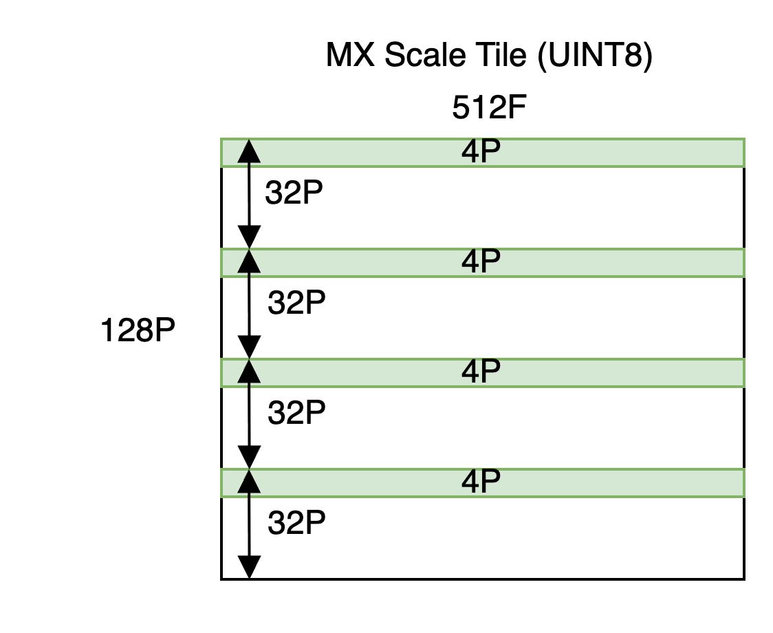
Notice the allocated shape is [128P, 512F] despite the underlying useful shape being [16P, 512F]. See the quantize_mx API for an example of how to improve memory usage by packing scales, from other quantized tensors, into the same allocation.

With this understanding we’ll state the space allocation rules for quantized MX scale tiles.

Unquantized Interleaved Data Tile = [P,F] BF16 in SBUF

If P <= 32 (Oversize optional)

MX Quantized Scale = [P//8, F//4] UINT8 in SBUF

If P > 32 (Oversize required)

MX Quantized Scale = [P, F//4] UINT8 in SBUF

Basic Matmul-MX#

This NKI example performs a single Matmul-MX using offline-quantized, max-sized input tiles. For simplicity, it assumes the MX data tiles in HBM already satisfy the layout requirements so they may be simply loaded straight into SBUF. The MX scale tiles require some shuffling. Note that subsequent examples, instead, show how to establish this layout yourself in SBUF.

@nki.jit(platform_target="trn3")
def kernel_offline_quantized_mx_matmul(stationary_mx_data, stationary_mx_scale, moving_mx_data, moving_mx_scale, mx_dtype):

  MAX_TILE_M = nl.tile_size.gemm_stationary_fmax  # 128
  MAX_TILE_K = nl.tile_size.pmax  # 128
  MAX_TILE_N = nl.tile_size.gemm_moving_fmax  # 512

  # View the input data as _x4 mx_dtype. This is done using an access pattern, specifying the target dtype and a simple
  # linear pattern.
  stationary_mx_data_hbm_x4 = stationary_mx_data.ap(dtype=mx_dtype, pattern=[[MAX_TILE_M,MAX_TILE_K],[1,MAX_TILE_M]], offset=0)
  moving_mx_data_hbm_x4 = moving_mx_data.ap(dtype=mx_dtype, pattern=[[MAX_TILE_N,MAX_TILE_K],[1,MAX_TILE_N]], offset=0)

  # Check that the input tiles are max-sized. This is merely for simplicity of the example but
  # smaller shapes are also supported.
  assert stationary_mx_data_hbm_x4.shape == (MAX_TILE_K, MAX_TILE_M)
  assert moving_mx_data_hbm_x4.shape == (MAX_TILE_K, MAX_TILE_N)

  # Load inputs directly from HBM to SBUF. Data is assumed to already have the
  # layout required by MX. Scales are assumed to be contiguous in HBM therefore we use
  # load_scales_scattered() to spread them across SBUF partition-dim quadrants, as is required
  # by Matmul-MX.

  stationary_mx_data_sbuf_x4 = nl.ndarray(stationary_mx_data_hbm_x4.shape, dtype=mx_dtype, buffer=nl.sbuf)
  nisa.dma_copy(src=stationary_mx_data_hbm_x4, dst=stationary_mx_data_sbuf_x4)
  stationary_mx_scale_sbuf = load_scales_scattered(stationary_mx_data_sbuf_x4, stationary_mx_scale)

  # Load moving
  moving_mx_data_sbuf_x4 = nl.ndarray(moving_mx_data_hbm_x4.shape, dtype=mx_dtype, buffer=nl.sbuf)
  nisa.dma_copy(src=moving_mx_data_hbm_x4, dst=moving_mx_data_sbuf_x4)
  moving_mx_scale_sbuf = load_scales_scattered(moving_mx_data_sbuf_x4, moving_mx_scale)

  # Allocate a tile in PSUM. This could also be float32.
  result_psum = nl.ndarray((MAX_TILE_M, MAX_TILE_N), dtype=nl.bfloat16, buffer=nl.psum)

  # Matmul-MX
  nisa.nc_matmul_mx(
    dst=result_psum,
    stationary=stationary_mx_data_sbuf_x4,
    moving=moving_mx_data_sbuf_x4,
    stationary_scale=stationary_mx_scale_sbuf,
    moving_scale=moving_mx_scale_sbuf
  )

  # Copy the PSUM result back to SBUF
  result_sbuf = nl.ndarray(result_psum.shape, dtype=nl.bfloat16, buffer=nl.sbuf)
  nisa.tensor_copy(src=result_psum, dst=result_sbuf, dtype=nl.bfloat16)

  # Store to HBM
  result_hbm = nl.ndarray(result_psum.shape, dtype=nl.bfloat16, buffer=nl.shared_hbm)
  nisa.dma_copy(src=result_sbuf, dst=result_hbm)

  return result_hbm

A few notes about the above example:

The MXFP_x4 packed data types are custom to NKI and are not supported in Torch. Therefore, we mimic the packed data using uint8 in Torch and simply view it as MXFP_x4 in the kernel, as shown.
The load_scales_scattered() helper function reads contiguously packed offline scales from HBM and spreads them across partition-dim quadrants.
The PSUM output tile is allocated with data type BF16 to indicate the desired output data type of the Matmul-MX. Note that Matmul-MX (nki.isa.nc_matmul) supports both BF16 and FP32 output dtypes.

Let’s also look at the host code which calls this kernel as all subsequent examples use the same structure.

def run_offline_quantized_matmul_mx_test(quantized_dtype):

  # Choose max tile-sizes for TensorE.
  M, K, N = 128, 128, 512

  print_test_header(f"OFFLINE_QUANTIZED_MX_MATMUL - stationary <{quantized_dtype.__name__}> @ moving <{quantized_dtype.__name__}>")

  setup_compiler_workdir(f"offline_quantized_mx_matmul")

  # Generate stationary MX tile. Note the scales will be packed contiguously here. The kernel will later load the scales into SBUF
  # in the required scattered fashion.
  st_unquantized_shape = (K, M*4)
  _, _, st_mx_data_x4, st_mx_scale = generate_stabilized_mx_data(quantized_dtype, st_unquantized_shape)

  # Generate moving MX tile
  mv_unquantized_shape = (K, N*4)
  _, _, mv_mx_data_x4, mv_mx_scale = generate_stabilized_mx_data(quantized_dtype, mv_unquantized_shape)

  # Call the Kernel. Perform matmul-mx: stationary_mx @ moving_mx
  output_kernel = kernel_offline_quantized_mx_matmul(
    torch.from_numpy(st_mx_data_x4).to(device),
    torch.from_numpy(st_mx_scale).to(device),
    torch.from_numpy(mv_mx_data_x4).to(device),
    torch.from_numpy(mv_mx_scale).to(device),
    quantized_dtype_to_x4_map[quantized_dtype]
  )

  output_kernel_np = output_kernel.cpu().float().numpy()

  # Generate the golden
  golden = nc_matmul_mx_golden(st_mx_data_x4, mv_mx_data_x4, st_mx_scale, mv_mx_scale, quantized_dtype, quantized_dtype)

  compare_and_print_results(output_kernel_np, golden)

The generate_stabilized_mx_data() helper function is used to generate MX data on the host. “Stabilized” means the data is randomly generated but injected with certain properties to allow for lossless quantization/dequantization, including constraining the data to be in the FP4/8 range. It conveniently returns MX data as ml_dtypes FP4/FP8, the same data packed into uint to mimic the MXFP_x4 packing (suitable for sending to a NKI kernel), MX scales, and a corresponding unquantized FP32 tensor. The input shape argument specifies the unquantized shape. The unquantized tensor is viewed as being in the required layout for MX operations. Therefore to generate an MX data tile of maximum size we must specify an unquantized free-dimension that is 4x larger. In this example the moving unquantized shape is [128P, 2048F] and the function will return a [128P, 512F] packed MX data tensor, as desired.
nc_matmul_mx_golden() is a utility to mimic the hardware’s Matmul-MX operation and is therefore useful for verifying the hardware output. It assumes the input tensors meet the SBUF layout requirements and the data tensor is packed to mimic MXFP_x4. Hence it can directly accept MX data generated by generate_stabilized_mx_data().
compare_and_print_results() uses numpy.allclose() to check data correctness and print the tensors to stdout.
Although this is a single-tile Matmul-MX, larger MX tensors can be multiplied by using the same tiling techniques shown in the non-MX Matrix Multiplication tutorial.

Quantize-MX + Matmul-MX#

Next we’ll replace one of the Matmul-MX inputs with a tile that we quantize on the VectorE using Quantize-MX. Again, it assumes the interleaved SBUF layout requirement is already satisfied. The source data for Quantize-MX must be in SBUF (cannot be in PSUM).

The two main changes in this example are:

The allocate_mx_tiles() helper function implements the data and scale tile allocation rules mentioned above.
load_scales_scattered() is again used for the stationary scales but is unnecessary for the moving scales since Quantize-MX will correctly spread the data across SBUF partition-dim quadrants.

# shape_unquantized represents the 2D unquantized SBUF shape with interleaved
# layout established (i.e. the shape immediately before calling Quantize-MX).
def allocate_mx_tiles(shape_unquantized, mx_dtype):
  assert len(shape_unquantized) == 2, f"shape_unquantized must have exactly 2 dimensions, got {len(shape_unquantized)}"

  P, F = shape_unquantized

  # Allocate data tile
  # Quantize-MX shrinks the free-dim by 4x because it packs 4 elements into 1.
  mx_data_sbuf = nl.ndarray((P, F//4), dtype=mx_dtype, buffer=nl.sbuf)

  # Allocate scale tile
  # Nominally the scale tile is sized (P//8, F//4) given that the scaling
  # group shape is [8P, 4F]. But when P > 32, the scales must be placed in the
  # partition-dim quadrant from which the corresponding scaling group originated
  # hence we must allocate the full P.
  if P <= 32: # Can store all scales in first p-dim quadrant.
    mx_scale_sbuf = nl.ndarray((P//8, F//4), dtype=nl.uint8, buffer=nl.sbuf)
  else: # Must oversize and spread across quadrants.
    mx_scale_sbuf = nl.ndarray((P, F//4), dtype=nl.uint8, buffer=nl.sbuf)

  return mx_data_sbuf, mx_scale_sbuf

@nki.jit(platform_target="trn3")
def kernel_on_device_quantize_matmul_mx(stationary_mx_data, stationary_mx_scale, moving_data_bf16, stationary_mx_dtype, moving_mx_dtype):

  assert moving_mx_dtype != nl.float4_e2m1fn_x4, "FP4 not supported by Quantize-MX"

  MAX_TILE_M = nl.tile_size.gemm_stationary_fmax  # 128
  MAX_TILE_K = nl.tile_size.pmax  # 128
  MAX_TILE_N = nl.tile_size.gemm_moving_fmax  # 512

  # View the input MX data as _x4 mx_dtype. This is done using an access pattern, specifying the target dtype and a simple
  # linear pattern.
  stationary_mx_data_hbm_x4 = stationary_mx_data.ap(dtype=stationary_mx_dtype, pattern=[[MAX_TILE_M,MAX_TILE_K],[1,MAX_TILE_M]], offset=0)

  # Check that the input tiles are max-sized. This is merely for simplicity of the example but
  # smaller shapes are also supported.
  assert stationary_mx_data_hbm_x4.shape == (MAX_TILE_K, MAX_TILE_M)
  # Note the factor of 4 on the N free-dim. This is unquantized data whose free-dim will be packed and
  # reduced by a factor of 4 during quantize_mx.
  assert moving_data_bf16.shape == (MAX_TILE_K, MAX_TILE_N*4)

  # Load stationary MX.
  stationary_mx_data_sbuf_x4 = nl.ndarray(stationary_mx_data_hbm_x4.shape, dtype=stationary_mx_dtype, buffer=nl.sbuf)
  nisa.dma_copy(src=stationary_mx_data_hbm_x4, dst=stationary_mx_data_sbuf_x4)
  stationary_mx_scale_sbuf = load_scales_scattered(stationary_mx_data_sbuf_x4, stationary_mx_scale)

  # Load moving BF16
  moving_bf16_sbuf = nl.ndarray(moving_data_bf16.shape, dtype=moving_data_bf16.dtype, buffer=nl.sbuf)
  nisa.dma_copy(src=moving_data_bf16, dst=moving_bf16_sbuf)

  # Allocate quantized moving tiles
  moving_mx_data_sbuf_x4, moving_mx_scale_sbuf = allocate_mx_tiles(moving_data_bf16.shape, moving_mx_dtype)

  # Quantize-MX. Scales will automatically be spread across partition-dim quadrants.
  nisa.quantize_mx(src=moving_bf16_sbuf,
                  dst=moving_mx_data_sbuf_x4,
                  dst_scale=moving_mx_scale_sbuf)

  # Allocate a tile in PSUM
  result_psum = nl.ndarray((MAX_TILE_M, MAX_TILE_N), dtype=nl.bfloat16, buffer=nl.psum)

  # Matmul-MX
  nisa.nc_matmul_mx(
    dst=result_psum,
    stationary=stationary_mx_data_sbuf_x4,
    moving=moving_mx_data_sbuf_x4,
    stationary_scale=stationary_mx_scale_sbuf,
    moving_scale=moving_mx_scale_sbuf
  )

  # Copy the PSUM result back to SBUF
  result_sbuf = nl.ndarray(result_psum.shape, dtype=nl.bfloat16, buffer=nl.sbuf)
  nisa.tensor_copy(src=result_psum, dst=result_sbuf, dtype=nl.bfloat16)

  # Store to HBM
  result_hbm = nl.ndarray(result_psum.shape, dtype=nl.bfloat16, buffer=nl.shared_hbm)
  nisa.dma_copy(src=result_sbuf, dst=result_hbm)

  return result_hbm

Please see the code package for the host code that calls this kernel.

SBUF Layout Using Strided Access#

Here we present two techniques for establishing the interleaved layout required for MX operations. Both produce the same result but have different performance tradeoffs. Therefore it’s useful to think of them as tools in a toolbox where you use the one that’s appropriate for your given situation.

It’s important to note that these techniques operate on unquantized tensors (BF16 in these examples) as the layout must be established before calling Quantize-MX. If you already have offline MX weights (already quantized), it’s suggested you establish the required layout offline so you may perform a direct load to SBUF.

The techniques are first explained then followed by a combined code example.

VectorE/ScalarE Strided Access#

Here we use either VectorE or ScalarE to write data to SBUF in the required layout. The simplest operation is a TensorCopy (shown below) but it’s usually more performant to apply the strided access pattern to some prior useful computation already occurring on these engines.

For completeness the example loads an HBM tensor to SBUF prior to rearranging the data on-device using an SBUF-to-SBUF TensorCopy. The load is needed for this to be a standalone executable example but in practice it’s expected your data would already be in SBUF from some previous operation. The TensorCopy strided access pattern is the key takeaway from this example.

Also note the TensorCopy source could be PSUM if you want to rearrange the data immediately after a prior matmul.

DMA Strided Access#

Here we DMA a tensor from HBM to SBUF using a strided access pattern. It’s conceptually similar to the above technique except the source of the copy is in HBM. This technique is typically significantly slower than on-device techniques but it can be useful in heavily compute-bound workloads where the DMA may overlap with compute.

Code#

This example demonstrates both techniques, selected by the use_tensor_copy argument. They are very similar but with slightly different read access patterns. It’s useful to refer to the above layout diagrams as you read this code as the reshapes and access patterns directly correspond.

def copy_data_strided(stationary_hbm, moving_hbm, use_tensor_copy: bool = True):

  # The HBM tensors have nominal shape [P,F]. Reshape into [4, P//4, F].
  # In other words, we divide the contraction axis into 4 "P" tiles since we'll eventually
  # need to read data from each tile and pack them together on SBUF.

  # These dimensions reflect the shape of each "P" tile.
  P_st = stationary_hbm.shape[0] // 4
  F_st = stationary_hbm.shape[1]
  P_mv = moving_hbm.shape[0] // 4
  F_mv = moving_hbm.shape[1]

  stationary_hbm_reshape = stationary_hbm.reshape((4, P_st, F_st))
  moving_hbm_reshape = moving_hbm.reshape((4, P_mv, F_mv))

  # Allocate SBUF tensors to store the strided result.
  # The shape is [P//4, F, 4] where the [P,F] is the shape of the unquantized input tensor.
  # In other words, we view the free-dim as having F_st/F_mv groups of 4 elements.
  # Taking 3D views of both the HBM and SBUF tensors allows for cleaner indexing.
  stationary_sbuf_strided = nl.ndarray((P_st, F_st, 4), dtype=stationary_hbm.dtype, buffer=nl.sbuf)
  moving_sbuf_strided = nl.ndarray((P_mv, F_mv, 4), dtype=moving_hbm.dtype, buffer=nl.sbuf)

  # Perform a TensorCopy to achieve the required layout.
  if (use_tensor_copy):

    # First load from HBM -> SBUF. Take "P" tiles from HBM and write them
    # contiguously (adjacent to each other) into the SBUF free-dim.
    # This load is not the focus of this example so its details are encapsulated in load_tensor_helper().
    # The SBUF shapes will be stationary_sbuf [P_st, 4, F_st], moving_sbuf [P_mv, 4, F_mv]
    stationary_sbuf, moving_sbuf = load_tensor_helper(stationary_hbm_reshape, moving_hbm_reshape)

    # Perform SBUF-to-SBUF TensorCopy to shuffle the data into the required MX layout.
    # Here are some tips on how to read this access pattern (AP).
    # .ap(pattern) = tuple of [step_size, count], right-most is the inner (fastest changing) dimension of the access pattern (AP).
    # The dst (*_strided) has no AP specified, meaning it is linearly written to.
    # To understand the src AP it's useful to refer to the SBUF Layout diagram in load_tensor_helper().
    # We read 1 element, then step F elements to the next tile, 4 times total. In other words, we gather a group
    # of 4 elements (one from each tile).
    # Then step 1 element and repeat the above F times to read an entire row of SBUF.
    # Then step to the next row of SBUF and repeat the above for all P rows of SBUF.
    # Note, this example is shown as a strided-read but it could be re-written as a strided-write, though it will be slower.
    # Secondly, the source tile can be in PSUM (i.e. the result of a prior matmul).

    nisa.tensor_copy(src=stationary_sbuf.ap(pattern=[[4*F_st, P_st], [1, F_st], [F_st, 4]], offset=0), dst=stationary_sbuf_strided)
    nisa.tensor_copy(src=moving_sbuf.ap(pattern=[[4*F_mv, P_mv], [1, F_mv], [F_mv, 4]], offset=0), dst=moving_sbuf_strided)

  # Perform a strided DMA to achieve the required layout.
  else:

    # Similar to TensorCopy, the we linearly write to stationary_sbuf_strided.
    # When reading from *_hbm_reshape, we read one element from each tile.
    # Then step 1 element and repeat the above F times, thereby reading one full row of HBM.
    # Then step to the next row of HBM and repeat the above P times.

    nisa.dma_copy(src=stationary_hbm_reshape.ap(pattern=[[F_st, P_st], [1, F_st], [P_st*F_st, 4]], offset=0),
                  dst=stationary_sbuf_strided)
    nisa.dma_copy(src=moving_hbm_reshape.ap(pattern=[[F_mv, P_mv], [1, F_mv], [P_mv*F_mv, 4]], offset=0),
                  dst=moving_sbuf_strided)

  # Return as 2D.
  return stationary_sbuf_strided.reshape((P_st, F_st*4)), moving_sbuf_strided.reshape((P_mv, F_mv*4))

See the code package for an example kernel that calls copy_data_strided() to establish the interleaved layout for stationary and moving tiles, quantize both, and perform a Matmul-MX.

Additional Tips#

It’s important to plan where in your design you’ll pay the cost of interleaving the data. Ideally you minimize the cost by finding existing, prior compute on which you can apply the strided access pattern. Or find existing compute against which you can overlap the interleave process. For offline MX weights prepare the layout offline on CPU so you may load the data to SBUF directly in a contiguous/unstrided fashion.
As with all compute on Neuron, it’s generally performant to spread it across multiple engines operating in parallel. Given that Quantize-MX runs exclusively on the VectorE a bit more care may be needed to alleviate VectorE contention by becoming familiar with operations that may be relegated other engines, like ScalarE.
The TensorE operates at double the clock frequency of VectorE, therefore Matmul-MX produces data at double the rate that Quantize-MX can consume it. It may seem that the TensorE could be back-pressured in a situation where a Matmul-MX quickly feeds a subsequent Matmul-MX (since you must Quantize-MX in between at half the speed), but that only happens for small tensors. Larger tensors require tiled matrix multiplication which inherently reuses input (quantized) tiles, allowing time for prior matmul output data to be quantized.

Matmul-MX supports PE-tiling (row-tiling only) where matmuls with a small (<= 64) contraction-dimension (partition-dimension) may be parallelized on the TensorE. This becomes more relevant for MX since a 4x-larger effective contraction-dimension is supported, meaning it’s useful for an MXFP_x4 contraction-dimension <= 64 or an equivalent unquantized contraction-dimension <= 256.

Executing the Code#

After downloading the tutorial code package to your Trainium3 Neuron environment, simply execute it as follows and observe the sample output.

$ python3 mx_toplevel.py

=====================================================================================
    OFFLINE_QUANTIZED_MX_MATMUL - stationary <float8_e5m2> @ moving <float8_e5m2>
=====================================================================================

Result shape: (128, 512)

np.allclose pass? True

Device Output:
[[0.02526855 0.59765625 1.15625   ] ... [-0.09033203 -0.10888672 -0.84375   ]]
...
[[ 0.25585938  0.18554688 -0.546875  ] ... [-0.71875    -0.6015625  -0.46484375]]

Golden:
[[0.02535721 0.5957752  1.1556101 ] ... [-0.09036541 -0.10906862 -0.8448767 ]]
...
[[ 0.2551025   0.1856966  -0.54681885] ... [-0.71797514 -0.6026518  -0.4641544 ]]


=========================================================================================
    OFFLINE_QUANTIZED_MX_MATMUL - stationary <float4_e2m1fn> @ moving <float4_e2m1fn>
=========================================================================================

Result shape: (128, 512)

np.allclose pass? True

Device Output:
[[-0.02038574  0.02648926  0.10351562] ... [-0.25        0.02404785  0.08154297]]
...
[[ 0.234375  -0.0456543  1.140625 ] ... [ 1.1015625   0.04833984 -0.17675781]]

Golden:
[[-0.02036181  0.02647817  0.10362364] ... [-0.24955288  0.02399684  0.08132255]]
...
[[ 0.23485765 -0.04565394  1.1424086 ] ... [ 1.0981529   0.04839906 -0.17722145]]


========================================================================================
    ON_DEVICE_QUANTIZE_MATMUL_MX - stationary <float4_e2m1fn> @ moving <float8_e5m2>
========================================================================================

Result shape: (128, 512)

np.allclose pass? True

Device Output:
[[-0.12792969  0.02685547 -0.19140625] ... [ 0.05883789 -0.01916504 -0.66796875]]
...
[[ 0.03198242 -0.24316406 -0.1640625 ] ... [ 0.06591797 -0.11914062  0.6015625 ]]

Golden:
[[-0.1284121   0.02687968 -0.19178611] ... [ 0.05882631 -0.01915852 -0.666565  ]]
...
[[ 0.03191248 -0.24304396 -0.16389877] ... [ 0.06606946 -0.11931092  0.60205466]]


======================================================================================
    ON_DEVICE_QUANTIZE_MATMUL_MX - stationary <float8_e5m2> @ moving <float8_e5m2>
======================================================================================

Result shape: (128, 512)

np.allclose pass? True

Device Output:
[[ 0.02832031 -0.29296875  0.04394531] ... [-0.13671875 -0.00704956 -0.47265625]]
...
[[ 0.03442383 -0.75        0.11572266] ... [ 0.86328125 -0.00735474  0.33007812]]

Golden:
[[ 0.02831857 -0.29297137  0.04390652] ... [-0.13685682 -0.00703458 -0.47168562]]
...
[[ 0.03451066 -0.7511592   0.11560257] ... [ 0.86369723 -0.00734489  0.3300762 ]]


================================================================
    COPY_STRIDED_TENSOR_COPY - <float8_e5m2> @ <float8_e5m2>
================================================================

Result shape: (128, 512)

np.allclose pass? True

Device Output:
[[ 0.56640625 -1.28125     0.26953125] ... [ 0.5859375   0.31054688 -0.60546875]]
...
[[ 1.2421875 -0.859375  -1.140625 ] ... [-0.06542969  0.11425781  0.6015625 ]]

Golden:
[[ 0.5663527  -1.2832397   0.26900524] ... [ 0.5861912  0.3109728 -0.6038357]]
...
[[ 1.2426924  -0.85944945 -1.1438001 ] ... [-0.0654989   0.11429967  0.6028823 ]]


============================================================
    COPY_STRIDED_DMA - <float8_e5m2> @ <float8_e5m2>
============================================================

Result shape: (128, 512)

np.allclose pass? True

Device Output:
[[ 0.32421875  0.43359375 -0.09814453] ... [ 0.82421875 -2.171875    0.71484375]]
...
[[-0.47070312 -0.734375    0.09765625] ... [ 1.328125   -1.09375    -0.32226562]]

Golden:
[[ 0.32461044  0.43410686 -0.09810834] ... [ 0.82437325 -2.1703691   0.71522826]]
...
[[-0.47003102 -0.733371    0.09745546] ... [ 1.3250915  -1.0969493  -0.32166338]]

MXFP Matrix Multiplication with NKI on AWS Neuron

Contents

MXFP Matrix Multiplication with NKI on AWS Neuron#

Before You start#

What is MXFP4/8 Matrix Multiplication?#

Layout and Tile Size Requirements#

Data Tensor#

Scale Tensor#

Basic Matmul-MX#

Quantize-MX + Matmul-MX#

SBUF Layout Using Strided Access#

VectorE/ScalarE Strided Access#

DMA Strided Access#

Code#

Additional Tips#

Executing the Code#